Building the Bandit Recommender
Assets & Materials doi: 10.5281/zenodo.21418033
| Realtime Recommendation Engine - Python Notebook (runs in browser). | |
| Bandit Fisher - Interactive simulation. A UCB bandit agent fishing in real time. | https://blog.vski.ai/fishing-demo/ |
| Bandit Fisher - Source Code. | https://vski.sh/x/bandit-fisher.git |
This is the practical companion to the earlier essay on contextual bandits. There we covered the math — greedy, ε-greedy, LinUCB, the optimism principle, and the ethical shape of the problem. Here we build the thing: state the problem the way a product team would, pick the machinery, and show what the greedy vs. UCB comparison actually looks like on a realistic workload. Read that essay first; this one assumes it.
The Fishing Simulator (the running analogy)
The companion fishing simulator is the cleanest way to see what a contextual bandit does, so it is worth establishing the analogy up front. The mapping is not literal, but it is precise where it matters.
| In the lake | In the recommender |
|---|---|
| The fisher | the recommender agent |
| The fish | the user (one user, one session) |
| Where the fish are hiding | the user’s hidden preference |
| The bait (colour, size) and cast location | the candidate item’s features |
| A cast | one recommendation decision — pick an arm |
| A bite | an engagement signal (click, dwell, completion) |
| No bite | the implicit signal that this was the wrong item |
| Casting again with a different bait | the next round of the loop |
The fisher cannot see the fish and does not know what bait they want. The only information is the rod: cast, feel whether the fish bites, adjust. That is the whole game — the agent never observes the user’s preference directly, only the reward signal from the item it chose to show. Every cast is a real interaction; you cannot cast a thousand times for free and pick the best.
In the simulator the fish move (the preference drifts), new baits become available, and the agent has to keep up. That is not a gimmick — it is the property that makes a static, pre-trained recommender useless and a bandit the right tool. The learning has to happen during the fishing.
The problem, in business language
A user lands on a page. You have a few hundred milliseconds to answer one question:
Given what I know about this user right now, which item should I show next?
There are no ratings. There is no clean "item → score" table. What you have
is a stream of implicit signals — how long they dwelt, whether they scrolled,
whether they clicked — and the item’s own features (tags, category, price band).
The fisher analogy holds all the way down: the bite is the click, the dwell
time, the completion. Never a survey response.
Three constraints make the obvious approaches fail.
1. No labels up front
There is no training set of "item → rating". The only way to learn what works
is to show items and watch the response. A supervised recommender needs a
fixed, labelled dataset to train on; here the labels only exist after you
act, and only for the action you took. The fisher learns the fish’s preference
by casting — not by reading a chart of past catches someone else logged.
2. The user is here now
Every shown item is a real interaction with a real customer. You cannot run an offline batch job overnight and come back tomorrow with a trained model — by then the user is gone, and the casts you “spent” exploring were real casts on a real fish. The learning has to happen during the session, in order, one decision at a time.
3. You must keep getting better
Tastes drift, new items arrive, the catalogue rotates. A model trained once and frozen goes stale. The fish move. The engine has to keep adapting for as long as it runs.
These three constraints — no labels, real-time, adaptive — are exactly the regime contextual bandits are designed for, and exactly the regime supervised recommenders are not. A supervised model trained on whatever you happened to show would learn your selection policy, not the user’s preference; a bandit is built to learn from actions it chose itself, which is the only honest way to learn from partial feedback.
Restated in bandit language (one paragraph — the previous essay covers the detail): at each round the environment presents an arm set of candidate items, each a feature vector; the agent selects ; the environment reveals only the reward of the chosen arm (partial feedback); the agent updates and repeats. The goal is to minimise cumulative regret — the running total of reward lost to suboptimal picks. Sub-linear regret means the agent is learning; linear means it is stuck. Everything below is judged by that curve.
The Hashing Trick
Before an agent can pick an arm, it needs to turn each item into a vector the
model can score. For a recommender the natural unit is the tag: an item
carries tags (minimalist, nature, food, portrait, …), and the user has
hidden preferences over tags. The question is how to map tags into
.
The naive answer — a one-hot column per tag, expanded every time the vocabulary grows — is a production nightmare. Every new tag changes the dimension, which means re-training, re-backfilling, re-deploying. The feature hashing trick kills all of that.
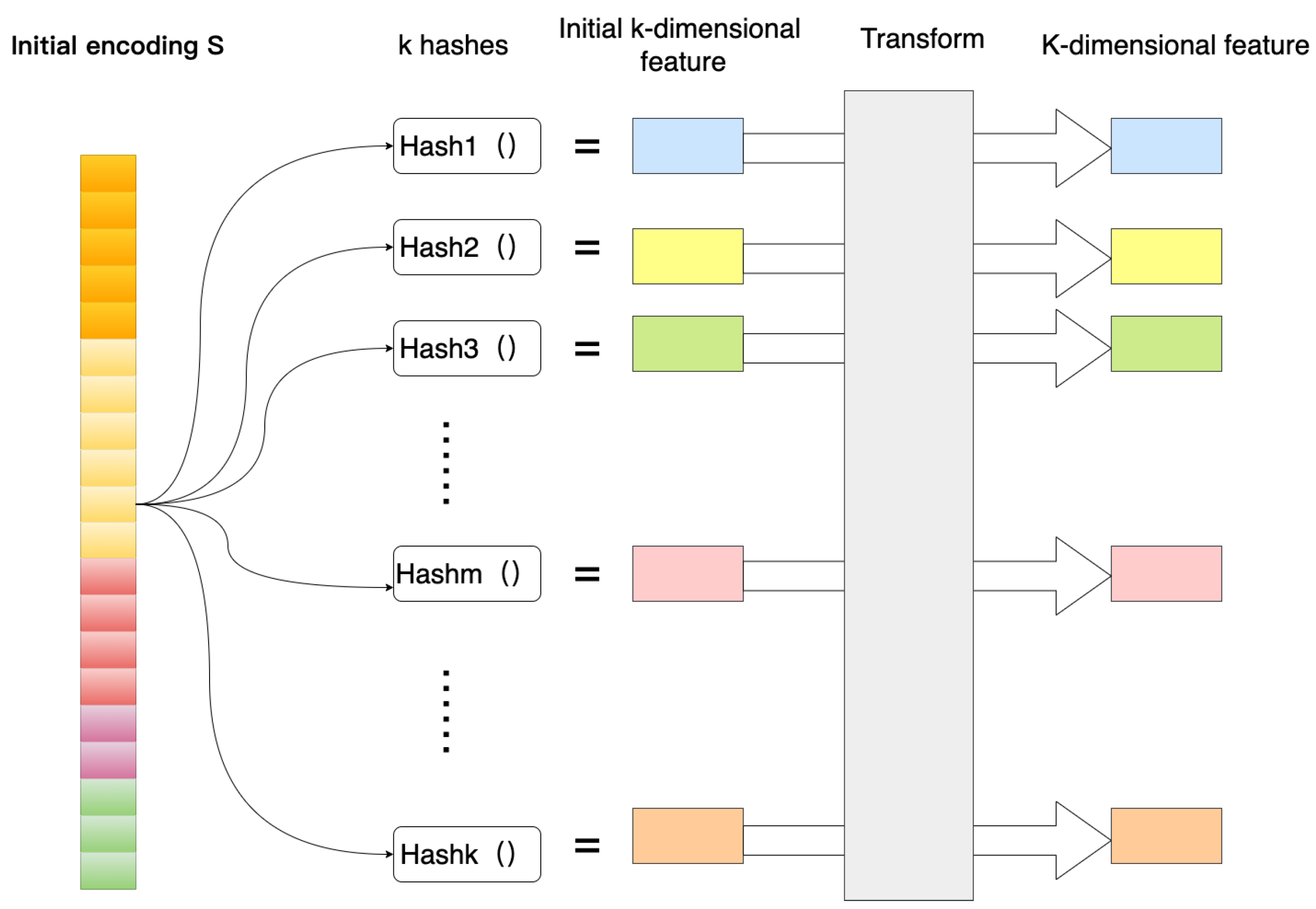
The construction
Each tag maps to a signed basis vector in a fixed :
- An index hash: , derived from (say) the tag’s md5 digest.
- An independent sign hash: , from a different bit of the same digest.
The tag’s vector is — a vector that is zero everywhere except at index , where it is . An item with tag set becomes the sum of its tag vectors, L2-normalised:
That is the whole featurizer. No vocabulary to maintain, no embedding table to train, no PCA to refit.
Why the sign hash matters
The sign hash is not decorative — it is variance reduction. Consider two
tags that collide (hash to the same index). Without signs, their contributions
always add: a collision between minimalist and ornate — opposite
preferences — would silently make the model think the user likes both equally,
a systematic bias. With random signs, colliding tags add half the time and
cancel half the time. The bias becomes zero-mean noise. You still pay for the
collision (a little signal is lost), but you pay it in noise, not in bias,
and noise is what regularisation and averaging are designed to absorb.
What you buy
- Fixed dimension. never grows as the vocabulary does. You pick it once ( in the engine, a few thousand in larger deployments) and the matrix algebra stays the same size forever.
- Streaming-safe. A new tag drops in at runtime with no state mutation, no
backfill, no pruning. The first time the agent sees
synthwaveit just hashes it and moves on. This is the property that makes the engine deployable as a single stateless loop — there is no feature store to keep in sync. - Interpretable inverse. Because the tag vectors are known and fixed, you can read the learned preference back as per-tag weights: project onto each tag’s hash direction, , and you get a readable list of what the agent thinks the user likes. The fisher can tell you “the fish wanted green bait, medium size” — not “the embedding was in cluster 47.”
What you pay
- Collisions. Two tags may hash to the same index. The expected collision count is for a vocabulary of tags — so the dimension is chosen by collision tolerance, not by explained variance (the criterion for embeddings). At with a small vocabulary, collisions are negligible; at too small for the vocabulary, the model silently degrades.
- Sign-cancellation. Two tags hashing to the same index with opposite signs cancel silently — an item carrying both loses the contribution of both. Measurable but usually minor at sensible .
- No semantic structure.
minimalistandminimalhash to unrelated indices. A CLIP embedding would know they are similar; the hash does not. This is the real trade-off: hashing is cheap and streamable but semantically blind, while embeddings are expressive but require a trained model and a frozen vocabulary.
The dimension choice is therefore a collision budget, not an information-theoretic one. Pick the smallest that keeps expected collisions below your tolerance, and stop. For a content recommender with a few dozen tags and a browser-deployable agent, is comfortable; the per-round cost is trivial and the collisions are essentially zero.
Greedy vs. UCB — the analytics
The previous essay established the three policies as a progression:
| Policy | Explore term | Where it explores |
|---|---|---|
| Greedy | none | nowhere |
| ε-greedy | random, probability | everywhere, uniformly |
| LinUCB | where the model is uncertain |
That table is the whole theory in three rows. The question the companion notebook answers empirically is: how much does the choice actually matter on a realistic workload? The setup: a synthetic catalogue of 200 items over a 16-tag vocabulary, hashed to ; a hidden user (likes minimalist, nature, serene; dislikes ornate, urban, dramatic); 8 candidate arms per round; 400 rounds; 12 random seeds, reporting median and inter-quartile range. Reward is a noisy linear score, shaped to .
The regret curves
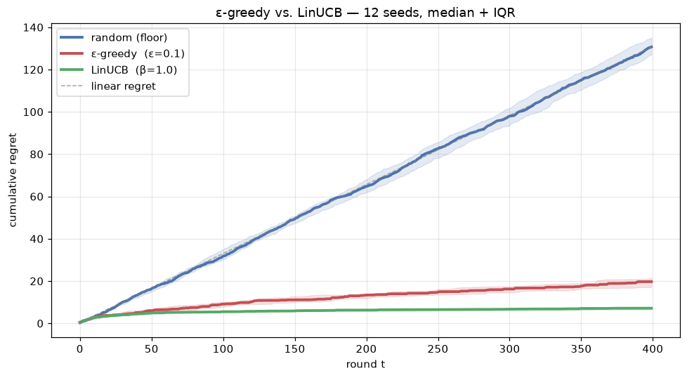
| Policy | Cumulative regret @ |
|---|---|
| Random (floor) | 130.7 |
| ε-greedy () | 19.7 |
| LinUCB () | 7.2 |
Two things to read off these numbers.
Shape, not just endpoint. LinUCB’s curve bends hard toward the horizontal — its slope drops as it learns, the signature of sub-linear regret. ε-greedy keeps a near-constant slope: it keeps paying the exploration tax every round, so its regret keeps climbing even after the model is good. Random, as a sanity check, is a straight line. The gap between a policy and the random line is the reward the engine earns by being smart.
Spread, not just median. LinUCB’s band across seeds is tight; ε-greedy’s is wider. ε-greedy’s fate depends more on whether its early random pulls happened to land on decent arms — the same contextual-freeze risk from the greedy case, softened but not removed. LinUCB’s directed exploration makes its trajectory reliable across users.
Why ε-greedy loses, structurally
This is not a tuning problem — it is the design. ε-greedy spends of every round on a uniformly-random pull, forever. Once the reward model is well-estimated, those random pulls are pure waste: the agent is showing known-worse items to a real user, for the rest of the session. Its regret cannot become sub-linear in because the exploration term never retires.
LinUCB spends its exploration budget only where the model is uncertain, and the bonus self-retires: every pull of an arm shrinks its bonus, so once an arm is well-observed the bonus collapses and the agent stops exploring it automatically. No to tune, no random pulls on known ground. The bonus is just the prediction standard error from ridge regression — STAT-101 wearing a bandit hat.
Convergence to the truth
A second diagnostic: how close does the agent’s estimate get to the hidden truth , measured by ? At the end of 400 rounds, LinUCB reaches , ε-greedy . Both are good — the linear model is the right model for this reward — but LinUCB gets closer, faster, because it spends its pulls where the estimate is still soft.
The interpretability check
Because the featurizer is hashing and the model is linear, projects cleanly back onto each tag. At the end of the run, the engine reports the user’s top-3 liked tags (minimalist, nature, serene) and top-3 disliked (ornate, dramatic, urban) — exactly the ground truth embedded in the simulator. No post-hoc explanation layer, no SHAP, no feature attribution. The fisher can tell you what the fish wanted.
When ε-greedy still wins
None of this makes ε-greedy wrong — it makes it the wrong tool for this regime. ε-greedy is the right tool when exploration is expensive and the model is already well-estimated: the post-exploration regime. By the time an e-commerce bandit goes live, the arms have usually been A/B tested upstream; pulling a known-worse arm “for exploration” means showing a known-worse promo to a paying customer. There, near-greedy () is the rational policy. LinUCB’s directed exploration is the right tool wherever the reward is genuinely unknown and worth learning — which is the regime a fresh recommender engine is born into.
The rest of the bandit family
Greedy, ε-greedy, and LinUCB cover the linear, continuous-reward case — which is most of what a content recommender actually needs. But the bandit family is larger, and the boundaries are worth knowing.
Thompson Sampling (linear-Gaussian). Same ridge-regression backbone as LinUCB, but instead of adding an optimism bonus, the agent samples a from the Gaussian posterior over each round and picks . This is probability matching: an arm is picked in proportion to the probability it is optimal. It has the same regret rate as LinUCB, often better constants, and production comparisons frequently favour it. The difference from LinUCB is philosophical — Bayesian “sample where you’re unsure” vs. frequentist “act as if the uncertain arm is as good as plausibly possible.” In practice both work well and the choice is often a matter of taste.
GLM-UCB (logistic bandits). When the reward is binary — click / no-click, convert / bounce — the linear-Gaussian model is mis-specified (Gaussian noise on a Bernoulli outcome, unbounded predictor on a probability). GLM-UCB passes the linear predictor through a logistic link and fits it by iteratively reweighted least squares (Newton’s method) at each round. Same regret rate as LinUCB, but no closed form: the per-round cost grows with the number of Newton steps, and there is a curvature constant that inflates when the sigmoid saturates. Worth adopting when the feedback signal is genuinely binary; overkill for continuous dwell time.
Neural bandits. For reward surfaces that are non-linear in the features
(tag conjunctions — “I like outdoor AND minimalist but not outdoor AND
busy” — thresholds, saturation effects), a linear model is wrong. Neural
bandits replace the linear regressor with a small network and derive the
exploration bonus from the network’s gradient or last-layer features. The
regret analysis is harder, the bonus is a black box, and the
explore/exploit trade-off is much more difficult to balance — the closed-form
geometry that makes LinUCB interpretable is gone. Use them when the reward is
genuinely non-linear and the linear model’s regret is unacceptable; the
fishing simulator, for instance, uses RBF features to fake non-linearity with
a linear bandit rather than reach for a neural one.
Adversarial bandits (EXP3 / EXP4). All of the above assume the reward distribution is stochastic and fixed. When an adversary controls the reward — click-fraud, bot traffic, a competitor gaming your auction — the optimism principle becomes a vulnerability (the adversary steers the agent toward arms that look uncertain). The adversarial family (EXP3 for non-contextual, EXP4 for contextual) replaces the regret guarantee with a worst-case one against an arbitrary sequence. Most recommenders do not need this; security and fraud detections sometimes do.
The practical pattern: start with a linear bandit (LinUCB or Thompson), move to GLM-UCB if the reward goes binary, reach for neural bandits only when the linear regret is demonstrably the bottleneck, and reserve the adversarial family for settings with an actual adversary. The same bandit loop — observe context, pick arm, observe reward, update — runs underneath all of them.
References
- Li, L., Chu, W., Langford, J. & Schapire, R. E. A Contextual-Bandit Approach to Personalized News Article Recommendation. (WWW 2010, arXiv.0146) — the original LinUCB paper, and the canonical reference for the algorithm used throughout the engine and notebook.
- Weinberger, K., Dasgupta, A., Langford, J., Smola, A. & Attenberg, J. Feature Hashing for Large Scale Multitask Learning. (ICML 2009, arXiv.2206) — the hashing trick, including the signed-hash variance-reduction argument.
- Abbasi-Yadkori, Y., Pál, D. & Szepesvári, C. Improved Algorithms for Linear Stochastic Bandits. (NeurIPS 2011, arXiv.2670) — the self-normalised tail bound behind LinUCB’s bonus and the regret guarantee.
- Filippi, S., Cappe, O., Garivier, A. & Szepesvári, C. Parametric Bandits: The Generalized Linear Case. (NeurIPS 2010) — GLM-UCB, the logistic extension for binary rewards.
- Chapelle, O. & Li, L. An Empirical Evaluation of Thompson Sampling. (NeurIPS 2011) — the production-scale comparison that established Thompson Sampling as a practical rival to UCB.
- Lattimore, T. & Szepesvári, C. Bandit Algorithms. Cambridge University Press, 2020. Freely available at https://banditalgs.com/ — the standard reference for the linear, GLM, and adversarial families surveyed above.
- Earlier essay in this series. Contextual Bandits and Their Ethical Use Cases — the math companion this post builds on (greedy vs. UCB policy design, the knob, the ethical shape of the deployment problem).
- Companion notebook. A Recommender Engine That Learns From Itself — the executable version of the ε-greedy vs. LinUCB comparison above, running entirely in the browser via Pyodide.