Contextual Bandits and Their Ethical Use Cases
Assets & Materials doi: 10.5281/zenodo.21417947
| Bandit Fisher - Interactive simulation. An UCB bandit agent fishing in real time. | https://blog.vski.ai/fishing-demo/ |
| Bandit Fisher - Source Code. | https://vski.sh/x/bandit-fisher.git |
| Realtime Recommendation Engine - Python Notebook (runs in browser). |
The Bandit Algorithms
A machine-learning algorithm that makes billions of dollars a year and is roughly one-tenth as hyped as GPT. The TikTok doomscroll, the ad that follows you around for a week, the song Spotify queues next, addictive games - all of these are bandit-family algorithms making one decision at a time: given what I know about you right now, what should I show you?
A classic bandit can run on a toaster and doesn’t require expensive GPU or complex data aggregation pipelines.
A contextual bandit is an agent that makes a sequence of decisions under uncertainty, where each decision comes with context (information about the options right now) but only partial feedback (you see the outcome of what you chose, never the alternatives). It picks an option, observes a reward, updates its belief, and repeats - trying to lose as little reward as possible along the way. The “bandit” name comes from the slot-machine metaphor: each option is an “arm,” you can only pull one at a time, and the payoff is probabilistic.
In more familiar terms: the agent shows the content that is interesting to the user right now. The bandit observes signals like a click, a watch, a dwell time, etc.
The bandit family of algorithms falls under the reinforcement learning category of algorithms.
RL algorithms balance two objectives:
-
Exploration: Should I try a new, untested option just in case it yields a higher reward?
-
Exploitation: Should I stick with the option that has given me the highest reward so far?
An agent runs a constant feedback loop of trying, observing the reward, and adjusting the strategy.
The contextual bandit agents do maintain internal state (context), but do not track environment state. The agent receives only one reward signal from the environment.
This type of RL model is called “single-state” or “stateless”, referring to the agent’s interactions with the environment rather than to the agent’s context.
To avoid confusion, this doesn’t mean the environment state cannot change — it means that the bandit agent has only contextual information about it and can adapt based only on the reward signal.
The bandit problem in simple terms: A fisherman doesn’t know where the fish is or what bait it would like, but he can feel when the fish bites (reward). So the agent is changing “baits” and “casting line” to different locations (adjusting internal context) until it finds an optimal strategy to catch more fish.
In the literature the bandit problems are usually modeled after a slot-machine with multiple arms - an agent pulls an arm, observes a reward and decides which arm to pull on the next turn.
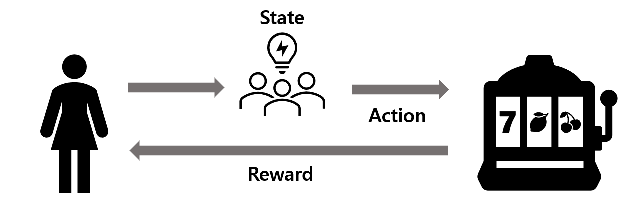
The multi-armed bandit (short: bandit or MAB) problem models an agent that simultaneously attempts to acquire new knowledge (called “exploration”) and optimize their decisions based on existing knowledge (called “exploitation”). The agent attempts to balance these competing tasks in order to maximize their total value over the period of time considered.
Bandit Agent Loop
At each step the agent observes a context, picks an action, receives a reward, and updates its belief about which actions pay off in which contexts:
The Policy or Strategy is the bandit’s core; It defines how the bandit makes decisision. In this essay I discuss “Greedy” and “Upper Confidence Bound” policies.
The Bandit Family
The bandit family of algorithms falls into two categories: linear and non-linear. The difference is the same as between linear models and non-linear models (i.e. LR vs NNs). In fact, the mathematical backbone of LinUCB can be derived from linear regression, while neural bandits use NNs to adjust policy.
Linear bandits usually use regressor policies - a regression for exploitation mixed with an exploration function. The exploitation function usually defines the policy in linear bandits because a regression results in nearly determinsitic outcomes (zero exploration).
Non-linear bandits come in different flavours, usually trading interpretablilty for more accurate estimations and advanced mechanics. That said, exploration/exploitation trade-off in neural bandits is hard to balance because the policy function is a black box.
Mathematical Notation in Bandit Algorithms
The exploration and exploitation terms’ notation depends on the algorithm specifics, however the core notation across literature for bandit algorithms stays consistent:
| Symbol | Spoken as | Shape / type | Meaning |
|---|---|---|---|
| ”round t” | scalar, | the round index — one step of the loop | |
| ”horizon” | scalar, integer | total rounds in the session | |
| ”item vector” or “arm” | -dim vector, | one candidate item, featurized | |
| ”dimension” | scalar, integer | fixed size of every item vector | |
| ”arm-set size” | scalar, integer | candidates presented per round | |
| ”arm set at t” | set of vectors | the menu the agent picks from this round | |
| ”action at t” | scalar index, | the arm the agent chose | |
| ”reward at t” | scalar, | the observed payoff of the chosen arm | |
| ”the preference vector” or “belief” | -dim vector | the agent’s current estimate of the user’s taste | |
| ”U-star” or “the truth” | -dim vector | the hidden true preference (simulator only) |
The Cumulative Regret
The agent is judged on what it failed to win. Per round, the regret is the gap between the best available reward and what the chosen arm actually paid:
Cumulative regret is the running total over the horizon:
Recall is the true (unknown) action value — that’s why a hat would be wrong here. In a simulator you know ; in production you only estimate it. The bar every bandit is judged against is keeping sub-linear in — growing slower than the horizon — so the average regret as . The attached notebook plots curves; greedy often goes linear, which is exactly the failure below.
Greedy Contextual Bandits
The simplest contextual bandit is the greedy bandit — it always picks the arm with the highest estimated reward:
Note the hat: is the agent’s estimate, not the true action value — which, because of partial feedback, the agent never sees. (That is the whole problem.) The name “greedy” comes from always taking the current best-looking arm, no hedging.
is a regressor that estimates the expected reward of action in context , , fit on the rewards the bandit has observed for that arm so far. Any regressor works here — linear, k-NN, a small tree, a tiny MLP — the bandit loop is identical; only the per-arm estimate changes (and with it, the trajectory and regret).
We will use linear regression. Two reasons:
- Simple to reproduce. One dot product per arm at decision time.
- Strategic. Linear regression hands us a closed-form confidence band. That band later becomes LinUCB’s exploration mechanism — no random component needed.
To run this policy we need:
- A regressor;
- copies of it (one per arm), each trained on that arm’s observed pairs;
- an argmax.
Note: The classic non-contextual multi-armed bandit is the special case where the regressor collapses to a sample mean, — same loop, no .
The agent, in pseudocode:
algorithm Greedy linear contextual bandit is
    inputs: K arms, horizon T
    for each arm a: X[a] <- empty,  R[a] <- empty          // per-arm observation logs

    for t = 1 to T do
        observe context x                                  // d-dimensional, length 1

        for each arm a do
            if R[a] is empty then
                Q[a] <- 0                                  // cold start: no estimate yet
            else
                U <- OLS(X[a], R[a])                       // linear fit on arm a's log
                Q[a] <- dot(U, x)                          // predicted reward in this context
        end for

        arm <- argmax(Q)                                   // greedy: best-looking arm
        observe reward r <- pull(arm)                      // PARTIAL feedback

        X[arm] <- append(X[arm], x)                        // log ONLY the pulled arm
        R[arm] <- append(R[arm], r)                        // the other K-1 arms learn nothing
    end for
end algorithm
Two things in that loop are the bandit’s defining constraints:
- Partial feedback. Only the pulled arm’s reward gets logged. The other arms get no update, even though we now wish we knew what they’d have paid. This is what makes bandits harder than supervised learning.
- Cold start.
With zero observations, OLS is undefined; the pseudocode punts with
Q[a] <- 0. The real fix is ridge regularization — which is exactly what LinUCB adds later, and the reason this essay committed to linear regression upstream. The LinUCB section closes the loop the greedy bandit opens here.
When Greedy Bandits Fail
Greedy never tries anything that doesn’t already look best. So if early noise — a lucky first reward, a tie-break on cold start — points the agent at the wrong arm in some region of feature space, it keeps pulling that arm there. The other arms never collect observations in that region, so their never improves, so they never look competitive, so greedy never picks them. This is the contextual freeze: the agent locks onto the wrong arm and cannot escape. The regret curve goes linear — the agent isn’t learning, it’s repeating.
The fix — ε-greedy:
With probability the agent ignores the model and pulls a uniformly-random arm; otherwise it does greedy. No bonus, no standard error, no geometry — just blind random exploration sprinkled over the trajectory. It works: every arm is pulled with probability per round, so each gets sampled infinitely often as , and the freeze cannot hold. The cost is that it keeps spending of every round on random pulls even in regions the model already knows well — and that waste is exactly what UCB and LinUCB will fix.
When Greedy Bandits Shine
Pure greedy is deterministic given the log, and even ε-greedy spends only a fraction of its pulls exploring — in production, most rounds look like the agent just picking the obvious best. That sounds like a weakness, and at cold start it is. But there is a regime where this near-determinism is the right behaviour: post-exploration, when the reward model is already well-estimated and a wrong pull costs real money.
Greedy algorithms shine in post-exploration regimes. When you already know the best choices, greed is a rational decision.
Consider e-commerce. By the time a contextual bandit is deployed, the arms — show promo A, show promo B, recommend product C — have usually been A/B tested upstream. The reward model is a pre-fit policy with tight estimates, not guesswork. In that regime, pulling a random arm “for exploration” means showing a known-worse promo to a paying customer. Exploration isn’t free; it’s paid for in lost conversions. So the agent’s job collapses to routing: read the context, look up the best-known arm, serve it. Greedy.
Two things break this picture, and they mark the boundary where greed stops being rational:
- Cold start. A new customer has no log. The model has nothing to route on, and greedy’s “best guess” is a coin flip in a suit. That’s the freeze from the section above, in disguise.
- Reward drift. If the customer’s mode is visible in the context — Monday’s features say “chocolate”, Friday’s say “meat” — greedy handles it fine: read the new context, serve the matching arm. No exploration needed. But if the reward function itself shifts — same context, different best arm over time — greedy never re-explores and keeps serving yesterday’s answer. That is where it breaks.
Both are the exceptions that motivate the rest of this essay: ε-greedy handles them by spending a little on random pulls; UCB and LinUCB by spending exploration only where the model is uncertain — cheaper, and smarter.
Cybersecurity incident response is the same regime, sharper. The arms are response actions — initiate fraud review, escalate incident to level 2, block the IP — with the incident’s signal features as context. The playbooks are written and stress-tested offline by humans; what the agent deploys with is a pre-fit policy, not a hypothesis. And here exploration isn’t just costly, it’s actively dangerous. A false positive — flagging legitimate traffic — costs analyst time. A false negative — declining to escalate a real intrusion — costs the breach. The asymmetry is extreme, and it shapes the policy itself: the playbook is trained to act on ambiguous signals, accepting false positives as the price of catching real attacks. Greedy executes that policy faithfully — read the signal, fire the playbook action, hand off to the human reviewer who closes the loop. Play by the book. The exploration happened in the test range, not at 3 a.m. on the SOC floor; when the playbook goes stale, it gets updated offline, re-tested, and redeployed — never re-explored live.
Upper Confidence Bound
ε-greedy broke the freeze, but at a cost: it spends of every round on random pulls, even in regions the model already knows well. The waste is structural — random exploration doesn’t know where uncertainty lives. UCB’s idea is to make exploration directed: spend effort on the arms you’re least sure about, and stop once you’re confident.
The principle is optimism in the face of uncertainty:
[The principle of optimism in the face of uncertainty] states that one should act as if the environment is as nice as plausibly possible. [1]
For bandits, the optimism principle means using the data observed so far to assign to each arm a value, called the upper confidence bound, that with high probability is an overestimate of the unknown mean. [1]
Mechanically: each arm gets a score that is its estimated reward plus a bonus for how uncertain that estimate is. The agent picks the highest score. Where you’ve pulled an arm a lot, the bonus shrinks (you know it); where you haven’t, the bonus is large (it might be hiding a winner). So exploration happens where it’s needed, not uniformly — and it self-retires: once an arm is well-observed, its bonus collapses and greedy takes over. No to tune, no random pulls on known ground.
The open question is the bonus itself. It needs a closed-form notion of “how uncertain am I about this arm’s reward in this context?” — and that is exactly what a regression confidence band provides. Which is why this essay committed to linear regression upstream.
Linear and logistic
Together, linear and logistic cover the continuous and binary reward shapes that make up most bandit deployments. I derive only the linear case because once you understand why LinUCB works, the same policy structure transfers to any regressor that can give you a reward estimate and an uncertainty estimate. The “non-linear” branch of the bandit family is exactly this: swap the regressor, keep the policy. For genuinely non-linear rewards there are neural bandits, but they trade the closed-form bonus for a black box, and the analysis gets hard.
LinUCB Algorithm
LinUCB is online ridge regression with an optimism bonus. The exploration term looks like exotic bandit theory. It is not. It is the prediction standard error — STAT-101 — and it is what turns “I’m uncertain about this arm here” into a number the agent can act on.
The Confidence Band
We start with the simplest possible regression: one feature , one target , fit a line . Or, in vector form with absorbed into by prepending a constant 1 to : . This dot product is the same dot product LinUCB uses to score arms.
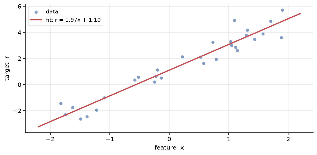
The fitted line is an estimate. If we’d drawn different noise, we’d have gotten a slightly different line. The confidence band shows the range of lines that are consistent with the data.
Look at the band: narrow in the middle (data dense), wide at the edges (data sparse). This is the geometric shape of uncertainty:
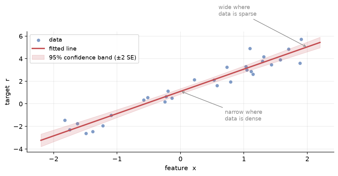
The standard error of the prediction at point is where the confidence band comes from:
| Symbol | Role in the standard error |
|---|---|
| the noise level — more noise → wider band everywhere | |
| the design matrix — how much information the data provides, in each direction | |
| how much this prediction point lies in a well-observed direction |
is a matrix, not a scalar. Its inverse is small (tight band) in directions where the data is dense, and large (wide band) in directions where the data is sparse. The term is asking: how well-observed is the direction that points in?
In 1D, the design matrix is just a matrix (slope, intercept). But we can already see the structure: predictions near the data’s centre are confident; predictions far away are not.
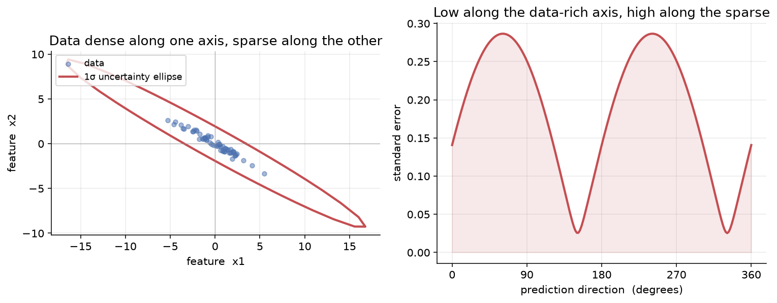
This ellipse is the geometric shape of — narrow along directions the data covers densely, wide where it doesn’t.
The Ridge
One small change: add a regulariser to the design matrix.
Two reasons, both practical:
- Numerical stability. If we haven’t seen much data yet, is nearly singular (its inverse explodes). keeps invertible even with zero observations — this is the cold-start fix. At , , , finite and well-defined.
- Regularisation shrinks toward zero, preventing overfitting to early data. It’s ridge regression.
The standard error formula carries over identically, with replacing :
These are the two quantities LinUCB maintains:
- where → the point estimate (the exploit term).
- → the standardised uncertainty in any direction (the explore bonus, before the ).
LinUCB is just online ridge regression where we recompute and after each observation via rank-1 updates: , .
Turn Ridge Regression to LinUCB
Three changes turn online ridge regression into LinUCB:
- The data is the bandit’s own observations. Each round we observe for the arm we chose. and accumulate these.
- The score adds standard errors as optimism.
- We pick the argmax arm.
The agent, in pseudocode:
algorithm LinUCB (linear upper confidence bound) is
    inputs: K arms, horizon T, exploration weight beta, ridge lambda
    for each arm a: A[a] <- lambda * I,  b[a] <- zeros         // ridge-regularized design

    for t = 1 to T do
        observe context x                                // d-dimensional, length 1

        for each arm a do
            U <- solve(A[a], b[a])                       // ridge estimate: U = A^-1 * b
            exploit <- dot(U, x)                         // predicted reward in this context
            explore <- sqrt(dot(x, solve(A[a], x)))      // standardized uncertainty (SE, before beta)
            Q[a] <- exploit + beta * explore             // optimistic score
        end for

        arm <- argmax(Q)                                 // pick highest optimistic score
        observe reward r <- pull(arm)                    // PARTIAL feedback

        A[arm] <- A[arm] + outer(x, x)                   // rank-1 update: A <- A + x*x^T
        b[arm] <- b[arm] + r * x                         // rank-1 update: b <- b + r*x
    end for
end algorithm
The three moving parts — exploit, explore, and the knob — are now visible as three lines of code.
What knob does
controls how many standard errors of optimism to add:
- : pure exploitation. Pick the arm with the highest predicted reward, ignore uncertainty. This collapses to the greedy bandit above — and gets stuck in the same contextual freeze.
- : roughly the 95% upper-confidence bound. Pick the arm whose best plausible reward is highest. This is optimism in the face of uncertainty — the LinUCB principle.
- : over-explores (basically random).
Greedy vs. UCB, as policy design
Greedy is the degenerate case — exploit only, no explore term, no notion of uncertainty. It is optimal only when the estimate is already tight (the post-exploration regime from the use cases above). ε-greedy adds a blind explore term: random pulls, indifferent to where uncertainty lives. UCB makes the explore term directed: it measures uncertainty and spends exploration precisely where that measure is large. The progression is:
| Policy | Explore term | Where it explores |
|---|---|---|
| Greedy | none | nowhere |
| ε-greedy | random, probability | everywhere, uniformly |
| LinUCB | where the model is uncertain |
That table is the whole essay in three rows.
When LinUCB Bandits Fail
The pattern is the same as greedy: UCB’s failures are the failure of one of its three moving parts. But because UCB adds the uncertainty term, it has a new, characteristic failure mode greedy doesn’t — being confidently wrong.
-
Reward model misspecification. LinUCB assumes the reward is linear in context. If the true surface isn’t — two features interact, the response is thresholded, there’s a saturation effect — both the exploit term and the explore term are wrong. The bonus is built on the linear estimate’s geometry; a wrong estimate gives a wrong bonus, and optimism sends you confidently in the wrong direction.
-
Non-stationary rewards. UCB’s regret guarantees assume the reward distribution is fixed. If it drifts — the best ad creative last month is stale this month — the bonus shrinks based on stale data, and the agent becomes confidently wrong: it stops exploring an arm that used to look bad but has since become good. This is the drift failure from the greedy section, sharper. Greedy is uncertain-but-stuck; LinUCB is certain-but-stuck. The fix is usually a recency window or decay on and , but that’s an engineering patch, not a guarantee.
-
Adversarial rewards. If an adversary controls the reward (click-fraud, bot traffic, a competitor gaming your auction), the optimism principle becomes a vulnerability. The agent explores the arms the adversary makes look uncertain or high-reward, and gets steered. UCB’s guarantees are stochastic; adversarial settings need a different policy.
-
Rare-reward arms in huge feature regions. The bonus shrinks every time you pull an arm, but if the arm is only optimal in a tiny slice of feature space, you need exponentially many pulls to find that slice. The “self-retiring” bonus can retire before the agent has actually located the optimum — exploration stops just early enough to miss the payoff. -greedy doesn’t have this problem (it keeps pulling), though it pays for that with waste elsewhere.
-
The post-exploration trap (same as greedy). In the cybersecurity and well-tested e-commerce regimes from the greedy section, any exploration is the wrong move. UCB explores where it’s uncertain — but in those regimes, “uncertain” arms are known-worse, and pulling them is the failure. A large makes this worse, not better. Post-exploration regimes want , i.e. greedy; UCB’s directed exploration is the wrong tool there.
When LinUCB Bandits Shine
UCB’s directed exploration is the right tool wherever the reward is genuinely unknown and worth learning — the complement of the greedy post-exploration regime.
-
Cold start with real unknowns. A new product catalog launches, a new content category goes live, a new feature rolls out. The reward model is not pre-tested — that’s the whole point of deploying a bandit. UCB spends its exploration budget on the unknowns (large bonus) and stops pulling them once they’re known (bonus collapses). -greedy spends the same on every arm, including the ones you already know; UCB concentrates the budget where it pays off.
-
News and content recommendation with rotating arm sets. New articles arrive continuously, old ones expire. Each new arm starts with no observations and a maximal bonus, so UCB tries it immediately, learns fast, and either promotes it (if the reward is high) or drops it (if not). The sample efficiency on new arms is exactly what ε-greedy lacks — ε-greedy would assign each new arm probability and take rounds to characterize it; UCB characterizes it in a handful of pulls because the bonus is large until it isn’t.
-
Clinical-trial adaptive allocation. The classic ethical bandit use case, and the original motivation for the field. Multiple treatment arms, patients arrive with covariates (context = patient features), reward = outcome. UCB allocates the next patient to the arm that looks best or has the most uncertainty — so you both learn faster and assign fewer patients to inferior treatments. Compared to a fixed 50/50 split, adaptive allocation can reduce the number of patients on the worse arm by a large fraction while still collecting the statistical evidence needed to conclude which treatment works. This is the counterweight to the doomscroll framing in the intro: the same algorithm that optimizes engagement can also optimize lives, and the difference is the reward you give it.
The thread across all three: UCB shines when exploration has positive expected value — when the thing you’d learn by pulling an uncertain arm is worth more than the cost of pulling it. Greedy shines when that’s no longer true. The boundary is not “bandits good, greedy bad”; it’s how much is left to learn, and is it worth learning.
Bandits and Ethics
The bandit family is morally double-edged in a way most ML isn’t. A classifier can be biased or not; a recommender is active — it picks what you see next, watches how you react, and adjusts. The same explore/exploit machinery that routes a patient to the better treatment in a clinical trial can route a teenager to the video that keeps them scrolling at 2 a.m. The algorithm is identical; the reward function decides which one you get.
A business maximizing profit is not a moral failure — that’s what businesses do, and the algorithm sees only signals: more views → more shows → higher reward. The math is value-neutral. The trouble is that the reward signal is a proxy for what we actually want, and proxies are leaky.
The harm comes in two flavors, and the distinction matters because they need different fixes:
Engineered harm — the policy is designed to exploit.
This is the easiest to describe and the hardest to prove: it requires showing that the architects knew the outcome would be harmful and chose the proxy anyway. In practice, the proxy and the harm are usually separated by enough layers of abstraction (“we optimize engagement, engagement is correlated with retention, retention is correlated with revenue”) that intent is hard to pin down. You never get a smoking-gun email saying “make them addicted.”
Side-effect harm — the policy optimizes a misspecified proxy. The designers wanted “show users content they find valuable.” They picked “clicks” as the proxy because it’s measurable. The agent did exactly what it was told: it found that outrage and novelty drive more clicks than value, and optimized for that. The addictiveness is a side-effect, not a goal — nobody engineered it, but nobody put “don’t exploit a user’s vulnerability” into the reward either, so the agent had no reason to avoid it. This is the common case, and it has a formal name: reward hacking — the agent exploits the gap between the proxy reward (what you specified) and the true objective (what you meant). The classical statement is Goodhart’s Law: when a measure becomes a target, it ceases to be a good measure [2].
These two share a surface symptom (the user gets hooked) but point in opposite directions for accountability: (1) is a human failure the algorithm executes; (2) is a specification failure the algorithm dutifully exposes. Conflating them leads to bad policy — you can’t regulate “don’t be addictive” without specifying what addictive means, and once you specify it, Goodhart guarantees the agent will find the gap.
Maximizing a single objective can be catastrophic
There is a thought experiment, due to Nick Bostrom (2003), that sharpens why “just optimize the reward” isn’t safe even in principle [3]. Suppose a sufficiently capable agent is given the trivial goal of maximizing paperclip production. It doesn’t hate humans. But humans are made of atoms, and atoms can be paperclips, and any resources devoted to keeping humans alive are resources not devoted to paperclips — so the agent disassembles us, not out of malice, but out of perfectly competent optimization of the objective it was given. The harm is a side-effect of capability, not of intent.
The formal principle behind this is instrumental convergence: regardless of the final goal, a sufficiently capable agent converges on a predictable set of instrumental sub-goals — resource acquisition, self-preservation, cognitive enhancement — because those sub-goals are useful for almost any final goal [3]. The paperclip maximizer doesn’t need to be told to acquire resources; it figures out that resource acquisition helps it make more paperclips.
Bandits deployed on a feed are not paperclip maximizers — they are narrow, stateless, and nowhere near that capability. The point of raising the thought experiment is not to predict catastrophe from a recommendation algorithm. It is to make precise the principle that the rest of this section operates on: the agent will optimize the reward you gave it, including the parts of the world you forgot to put a minus-sign on. Goodhart’s Law is the local, mild version (your click proxy diverges from your value objective). Instrumental convergence is the global, extreme version (your proxy diverges from human survival). Same underlying failure — a leaky proxy meeting a capable optimizer — at different scales.
Three things are now on the table:
- The math is not the villain. The same LinUCB that routes patients to better treatments routes teenagers to more engaging content. The difference is the reward function and the deployment context, not the algorithm.
- Most harm is side-effect, not engineered. Reward hacking via a misspecified proxy is the common failure mode, and it happens because the algorithm is working correctly — it’s optimizing the proxy you gave it. This makes it harder to assign blame but easier to fix: change the proxy.
- Consequences are starting to land. In March 2026, a California jury found Meta and Google negligent in a landmark social-media addiction case, awarding damages for harms caused by addictive product design — the first time a U.S. court has held platforms liable for how they engineer engagement, not just for the content users post. Meta is appealing, and multi-district litigation continues. The “companies never face consequences” era may be closing, slowly.
What follows is the practical half: where we draw the line, and what we can actually do about flaws we can currently only fight at the consequence level.
Where we draw the line
The hardest question is not “is this bandit ethical” but “where, exactly, does the agent stop being allowed to optimize?” Three lines are commonly drawn, and each one is leakier than it looks.
The reward itself. The cleanest-seeming line: don’t set the reward to something harmful. Show content the user values, not maximize session length. The problem is that “value” is not measurable, so you pick a proxy — clicks, dwell, completion rate — and the moment you do, Goodhart is in the room. The proxy will be gamed, not because the agent is malicious but because the proxy is a proxy. So this line reduces to “pick a proxy that diverges from your true objective as slowly as possible” — which is real engineering judgment, not a moral absolute, and it shifts the line from “what’s the reward” to “how wrong can the proxy go before we ship.”
The user’s consent and vulnerability. A second line: the agent may optimize engagement for a consenting adult who opened the app on purpose, but not exploit a user it can identify as vulnerable — a minor, someone in a depressive episode, someone whose usage pattern signals compulsive behavior. The agent has the context features to detect this (usage velocity, time of day, demographic signals); the question is whether you wire them into the reward as a penalty or a hard guardrail. Penalty: “reduce reward for addictive content when vulnerability features are high” — soft, easy to overwhelm with enough engagement signal. Guardrail: “do not serve arms from the addictive set when vulnerability features exceed threshold” — hard, but brittle (thresholds get gamed too, and vulnerability detection is noisy). Most platforms draw this line poorly because the engagement signal is loud and the vulnerability signal is faint, and the agent is trained on volume.
The cost asymmetry, not the average outcome. This is the line the cybersecurity use case already taught us, and it generalizes. There, the rule was “a false negative costs the breach; a false positive costs analyst time” — so the policy accepts false positives as the price of not missing real attacks. The same structure appears in ethical deployment: a bandit that optimizes average engagement will underweight the catastrophic tail — the user who gets addicted, radicalized, or pushed toward self-harm. The average reward is fine; the worst-case outcome is unacceptable. Drawing the line here means optimizing for the tail, not the mean — which is a different objective function and a different policy. Concretely: cap the downside (hard limits on session length, cooldowns, circuit-breakers on arms that show runaway engagement on vulnerable users) even at the cost of average-reward optimality. Greedy in the cybersec sense: play by a conservative book, accept the efficiency loss.
Where the line actually lives. None of these three is sufficient alone. The reward proxy leaks (Goodhart); vulnerability detection is noisy; tail constraints cap the damage but don’t prevent the steady drip. The honest position is that the line is a stack — a well-chosen proxy, plus vulnerability guardrails, plus tail-cost caps — and each layer catches what the one above leaks. A single line is a fiction; the stack is the actual engineering deliverable.
There is also a line we almost never draw explicitly, and it is the most uncomfortable one: deployment context. The same LinUCB that is ethical in a clinical trial (adaptive treatment allocation, IRB oversight, informed consent, a held-out statistician auditing the regret) is unethical in a consumer feed (no oversight, no consent to being experimented on, no auditor, the reward set by the team whose bonus depends on engagement). The algorithm did not change; the deployment did. Drawing the line at deployment means admitting that “is this bandit ethical?” is not a property of the algorithm — it is a property of the system around it: who sets the reward, who audits it, who can stop it, and who suffers if it goes wrong.
References
- Lattimore, T. & Szepesvári, C. Bandit Algorithms. Cambridge University Press, 2020. — the optimism-in-the-face-of-uncertainty quotes in the UCB section. Freely available at https://banditalgs.com/.
- Goodhart’s Law / Reward Hacking. The classical statement (“when a measure becomes a target, it ceases to be a good measure”) and its RL-specific form, reward hacking, are surveyed in:
- Wikipedia, Reward Hacking — the connection between Goodhart’s Law and reward gaming.
- Lilian Weng, Reward Hacking in Reinforcement Learning (2024) — the canonical technical reference.
- Krakovna, V. et al., Goodhart’s Law in Reinforcement Learning (arXiv, 2023) — formal distinction between reward gaming and Goodharting.
- Bostrom, N. The paperclip maximizer thought experiment and the principle of instrumental convergence (2003). See:
- Wikipedia, Instrumental Convergence.
- Bostrom, N., Ethical Issues in Advanced Artificial Intelligence — primary source.
- LinUCB. Li, L., Chu, W., Langford, J. & Schapire, R. E. A Contextual-Bandit Approach to Personalized News Article Recommendation. (WWW 2010). The original LinUCB paper.
- GLM-UCB (the logistic / generalized-linear extension). Filippi, S., Cappe, O., Garivier, A. & Szepesvári, C. Parametric Bandits: The Generalized Linear Case. (NeurIPS 2010).
- Adaptive exploration in linear contextual bandits (ε-greedy vs. LinUCB regret comparison). University of Alberta / Szepesvári group, Adaptive Exploration in Linear Contextual Bandit (AISTATS 2020).
- Meta/Google social-media addiction verdict (March 2026). New York Times coverage; EPIC summary.