Quartiles, Ridge, and Lasso

The first is quartiles — a way to describe a distribution that survives weird data. The other two, Ridge and Lasso, are regularisation methods — ways to keep a regression model from fitting the noise in its training data. All three are the kind of thing a course mentions in week two and never comes back to, and all three are the kind of thing that, ten years later, decides whether a model you shipped is robust or embarrassing.

I will use a single running example: a panel of 60 firms, each described by its sector, size, CEO profile, and a handful of security metrics. Two questions hang over the panel. Given how many breach attempts a firm absorbs, how many will actually succeed? — a regression problem. And the thing that makes the answer trustworthy is exactly the thing this essay is about: describing the data honestly before modelling it, and restraining the model after.

The throughline is restraint. Quartiles restrain the influence of outliers on our description of data. Ridge and Lasso restrain the influence of noise on our estimate of the model. Different objects, same instinct: don’t let the extremes dictate the centre.

Quartiles — describing data that misbehaves

Suppose I ask you how many successful breaches a typical firm in the panel suffered. The lazy answer is the mean: 22.6. The mean is also the wrong answer, because the distribution is not symmetric — a handful of firms in Hospitality got hammered, and the mean is dragged up by them. A firm picked at random is more likely to be near the median (18) than near the mean, and the gap between those two numbers is itself a signal: it tells you the data is skewed.

Quartiles cut the sorted data into four equal quarters and report the three fence posts between them:

cut	name	meaning
25th percentile	Q1	a quarter of firms are below this
50th percentile	median (Q2)	half below, half above
75th percentile	Q3	three quarters below

For the breach data those posts are Q1 = 3, median = 18.5, Q3 = 32. The range that matters is not min-to-max (that would be 0 to 100, dominated by extremes) but the interquartile range, $\text{IQR} = Q3 - Q1 = 29$. The IQR is the middle fifty percent of the data — where a typical firm actually lives.

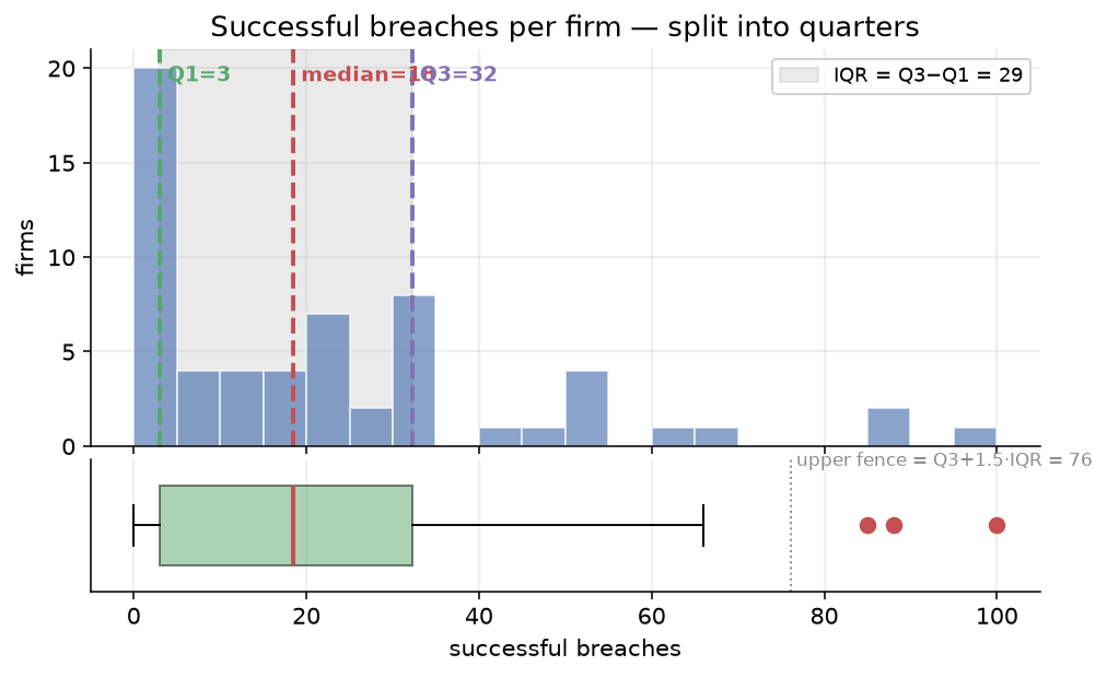
The picture makes the point. The histogram is lopsided; the boxplot beneath it draws the IQR as a box, extends “whiskers” to the last non-extreme points, and flags the three firms at 85, 88, and 100 as outliers. The outlier rule is mechanical and conservative: anything beyond $Q3 + 1.5 \cdot \text{IQR}$ (or below $Q1 - 1.5 \cdot \text{IQR}$) is flagged. For this data the upper fence is $32 + 1.5 \times 29 \approx 76$, so the three firms above it stand out.

Why the 1.5? It is a convention, tuned so that, if the data were perfectly normal, roughly 0.7% of points would be flagged as outliers by chance. So the rule is a “this would be surprising under a normal distribution” detector, not a philosophical statement about what an outlier is. Use it as a flag, not a verdict.

The reason quartiles matter here is practical. Before fitting anything, I want to know: is the target symmetric or skewed? Are there points that will dominate a squared-error loss? Which firms are the unusual ones? Quartiles answer all three without assuming any distribution, and they survive the outliers that would corrupt a mean and standard deviation. That is the whole pitch: description that does not break when the data does.

Ridge — shrinking coefficients without silencing them

Now the model. We want to predict successful breaches $y$ from a vector of inputs $x$ (breach attempts, sector, size, and so on). Ordinary least squares (OLS) picks the coefficients $\beta$ that minimise the squared error on the training data:

$$\hat{\beta}_{\text{OLS}} = \arg\min_{\beta} \ \| y - X\beta \|^2$$

OLS has a property that is both its charm and its danger: it will move coefficients as far as they need to go to shave the last bit of training error. On 60 rows with a dozen features, that is too much freedom. The fit is great on the rows it has seen and wobbly on the rows it hasn’t — the textbook high-variance, low-bias failure. The model has overfit: it learned the noise as if it were signal.

Ridge regression adds a penalty for coefficient size:

$$\hat{\beta}_{\text{Ridge}} = \arg\min_{\beta} \ \| y - X\beta \|^2 + \alpha \|\beta\|_2^2$$

The second term, $\alpha \|\beta\|_2^2 = \alpha \sum_j \beta_j^2$, is the L2 penalty. It says: fit the data well, but keep the coefficients small. The knob $\alpha \geq 0$ trades the two goals against each other. At $\alpha = 0$ you recover OLS. As $\alpha$ grows, every coefficient is pulled toward zero, and the fit loosens. You give up a little bias for a lot of variance reduction.

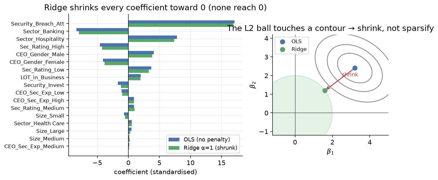
The left panel shows it directly. Every blue OLS bar is matched by a shorter green Ridge bar — the dominant coefficient (breach attempts, around +17) barely moves, but the smaller ones shrink noticeably. Nothing reaches zero. That is Ridge’s signature: shrink all, silence none. The right panel is the geometry behind it. The grey ellipses are contours of equal training error, nested around the OLS solution (blue). The green circle is the L2 constraint, $\|\beta\|_2 \leq t$, centred at the origin. Ridge’s solution is the point where the smallest contour just touches the circle — the closest you can get to OLS without leaving the allowed region. Because a circle is round, it touches a contour on its side, never on an axis. Every coefficient stays nonzero.

That roundness is the whole story. The L2 ball has no corners, so the tangent point is generically off-axis, which means Ridge shrinks coefficients smoothly but cannot perform feature selection. What you get for that is stability: Ridge has a closed-form solution, plays well with correlated features (it spreads weight across them instead of picking one arbitrarily), and its coefficient paths are continuous in $\alpha$. On the breach data it lifts the cross-validated $R^2$ from 0.767 (OLS) to 0.776 ($\alpha = 1$) — a small gain in mean, but more importantly a tighter spread across folds. That is the regularisation bargain: less flash on the training set, more honesty on data it hasn’t seen.

Lasso — the same idea, with a different shape

Lasso changes one symbol, and that change does all the work. Replace the L2 penalty with an L1 penalty:

$$\hat{\beta}_{\text{Lasso}} = \arg\min_{\beta} \ \| y - X\beta \|^2 + \alpha \|\beta\|_1, \qquad \|\beta\|_1 = \sum_j |\beta_j|$$

The penalty now grows with the absolute sum of coefficients, not the squared sum. That sounds like a small accounting change. It is not. The L1 penalty drives some coefficients exactly to zero, which L2 never does. Lasso is therefore two tools in one: a regulariser and a feature selector.

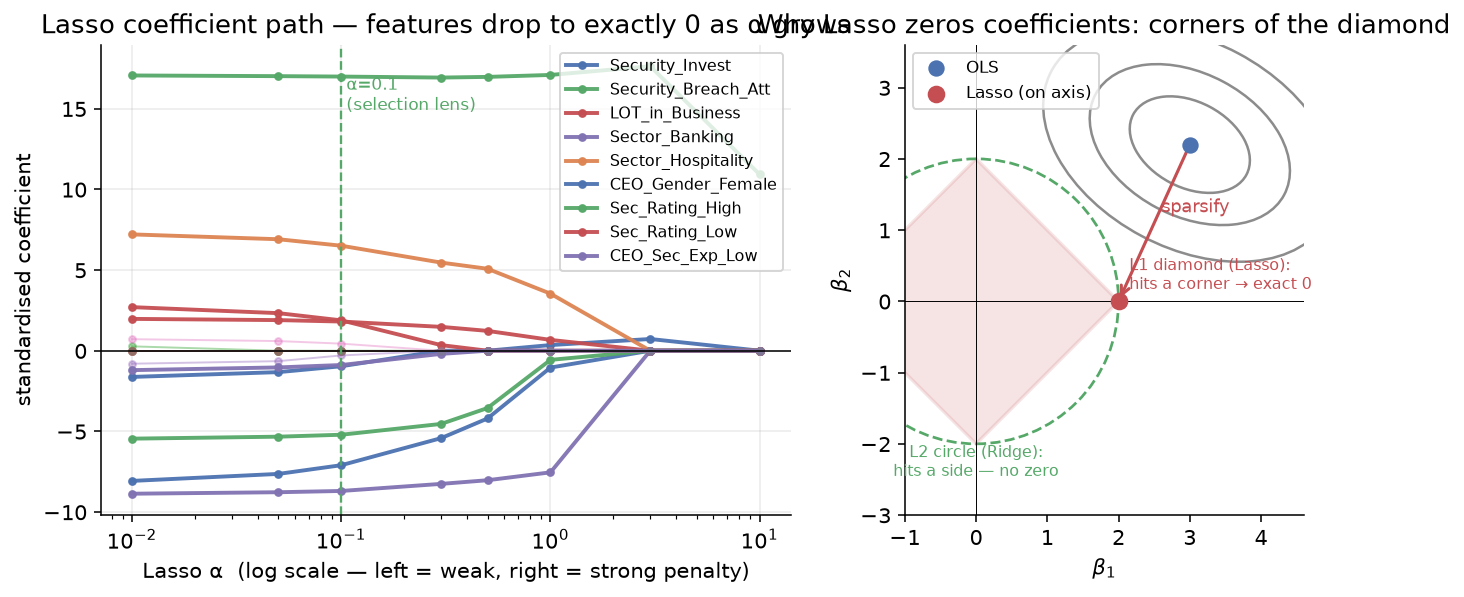
The left panel shows the effect. Each line is a feature’s coefficient as $\alpha$ increases. Reading left to right (weak to strong penalty), the small coefficients hit zero first — Size, CEO_Sec_Exp, Security_Invest vanish by $\alpha \approx 0.3$ — while the dominant signal (Security_Breach_Att, holding at +17) survives almost to the end. By the time $\alpha$ is large, only one or two features remain. That is the model telling you which inputs matter. For an underwriter pricing breach risk, that is a deliverable: invest in measuring breach attempts and sector accurately; the CEO-experience questionnaire is not pulling its weight.

The right panel explains why the zeros happen. The grey contours are the same RSS curves as before. But the constraint region is now the red diamond $|\beta_1| + |\beta_2| \leq t$ — the L1 ball. Diamonds have corners, and the corners sit on the axes, where one coefficient is exactly zero. When the smallest RSS contour expands to meet the diamond, it almost always hits a corner first. So the Lasso solution lands on an axis, and the feature on that axis is silenced. The dashed green circle shows the contrast: Ridge’s round L2 ball touches a contour on its side, so it shrinks without zeroing. The shape of the penalty region is the behaviour of the model.

The trade-off, compared to Ridge, is that Lasso is less gentle with correlated features. Where Ridge spreads weight across two correlated predictors, Lasso tends to pick one and zero the other — a choice that can be unstable across samples. And Lasso has no closed-form solution; it needs an iterative optimiser. But when you have more candidate features than the data can support, that sharp-edged sparsity is exactly the property you want. On the breach data, a Lasso at $\alpha = 0.1$ keeps the same predictive accuracy as OLS while dropping five features outright — a simpler model that is easier to defend, for free.

Conclusion — three restraints, one instinct

Stack the three tools next to each other and a pattern appears.

tool	what it restrains	how	what you get
Quartiles	outliers in description	report ranks, not moments	a summary that survives skew
Ridge	coefficient size in estimation	L2 penalty, smooth shrink	stability, no zeros
Lasso	coefficient count in estimation	L1 penalty, sharp sparsity	a smaller, explainable model

Quartiles restrain the data’s extremes from dictating our summary. Ridge and Lasso restrain the model’s coefficients from chasing noise. The mechanism differs — rank-based cuts, a squared penalty, an absolute penalty — but the instinct is the same: don’t let the loudest inputs set the whole story.

The breach-data example ties them together. Quartiles showed the target was skewed and flagged three firms as outliers, which told us to be careful with a squared-error loss and to check those firms’ leverage. Ridge, applied after, trimmed the model’s variance enough to beat OLS out-of-sample. Lasso, applied as an explanation tool, confirmed that almost all the signal lives in one feature (breach attempts) plus a couple of sector indicators — so the underwriter knows where to invest in data quality and where to stop collecting. None of these is a model on its own; together they are the difference between a fitted line and a defensible answer.

Two practical notes for actually using these. First, the penalty $\alpha$ is a dial, not a switch, and the right setting is found by cross-validation, not by intuition — try a grid of values and keep the one that holds up on held-out folds. Second, Ridge and Lasso are not rivals but colleagues. When features are correlated and you want stability, reach for Ridge. When you have too many features and need a shortlist, reach for Lasso. There is even a middle path, Elastic Net, that blends both penalties and takes the good of each — useful when you suspect groups of correlated features matter together but the set is still too large.

Most modelling failures are not failures of the algorithm — they are failures of restraint. A mean used where a median was needed; an OLS fit given enough freedom to memorise the noise; a feature set left unpruned because no one asked which inputs mattered. Quartiles, Ridge, and Lasso are three cheap, old, unglamorous ways to exercise that restraint. They will not make a model clever. They will stop it from being foolish, which is usually the harder part.