A Non-Linear Online Bandit for Set-Compatible Collection
Assets & Materials doi: 10.5281/zenodo.21534769
| Kitchen — Research Notebook. The binary pickup/skip classifier with tree head, linear foil, and EWMA-ECDD drift detector, trained end-to-end. | |
| Online Demo: Non-Linear Set Collection Agent | https://blog.vski.ai/kitchen/ |
| Online Demo (Source Code) | https://vski.sh/x/kitchen |
| Reflex Bandit: Active Exploitation (Predecessor — single-token, additive reward) | https://blog.vski.ai/posts/bandits-active-exploitation/ |
Online bandits fall into two regimes. The active explorer has noisy sensors and a largely unknown world; its job is to find out where reward is. The active exploiter has noiseless sensors but does not know what they mean — tokens are fixed, the world’s shape drifts, and the agent must learn the reflex each shape demands. A linear bandit handles both regimes well when the value of a thing is independent of every other thing: it learns per-token weights, recommends accordingly, and converges in a handful of episodes.
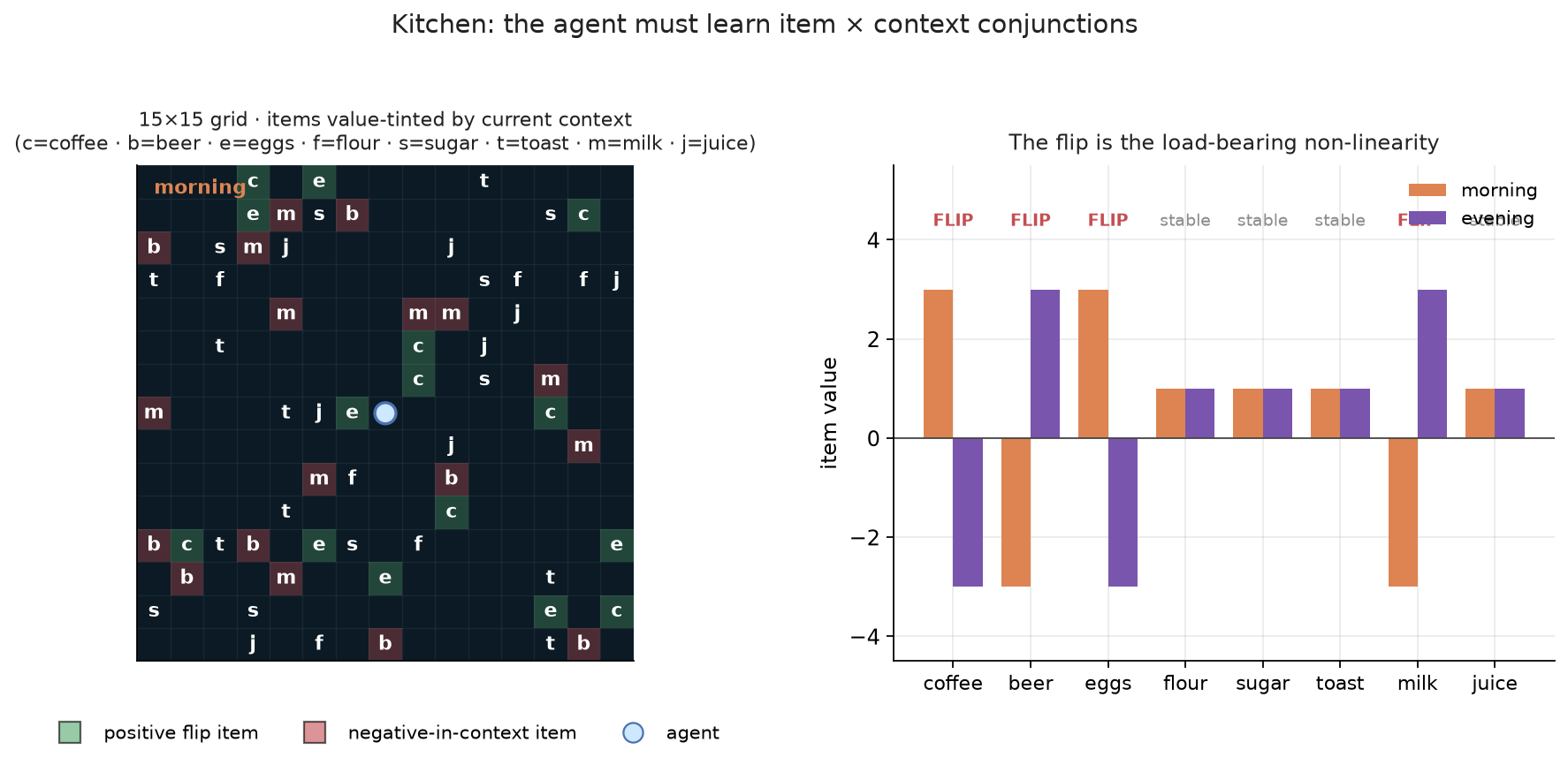
This post is about the regime just past that boundary. The value of a thing now depends on context — coffee is positive in the morning and negative in the evening; beer the opposite. The “good” set flips with the context. A linear value head over item and context features provably cannot represent this dependence, because its dot product has no item×context cross term. Its best estimate of coffee’s value is the average across contexts, which is zero — wrong by three in both directions.
The fix is not a neural network. Non-linear does not mean neural. It
means interaction-aware. And the cheapest interaction-aware function
class available — a tree ensemble — represents exactly the low-order
conjunctions (item=coffee AND ctx=morning) that two or three
axis-aligned splits enumerate for free. No embedding, no gradient, no
last-layer Bayesian reweighting.
The agent in this post makes one learned decision — pickup or skip — per item it encounters, walking freely between items via a fixed BFS policy. A linear foil runs over the identical feature vector, identical training data, identical loop — only the function class differs. When the linear foil plateaus at chance and the tree clears 0.84, the non-linearity is load-bearing. That collapse, on the same data, is the load-bearing finding.
The regime
Set-compatible collection is the right framing whenever three conditions hold simultaneously.
| Condition | What it means | Why it matters |
|---|---|---|
| Item values interact | The reward of collecting A depends on external context, or on whether B is already collected. | An additive value head — linear in the features — provably cannot represent this. |
| Context flips value | Some item is positive in one context and negative in another (morning vs evening). | The model must learn a conjunction (item AND context), not a per-item weight. |
| Selection is forced | The agent cannot collect everything; it must choose a subset. | Indiscriminate collection is punished; the agent must discriminate. |
When all three hold, a linear value head plateaus at chance. The reason is structural and worth stating precisely.
A linear model over a feature vector computes . Suppose the feature vector contains a one-hot for the
encountered item (item-coffee = 1) and a one-hot for the time of day
(ctx-morning = 1). The linear model has a weight
and a weight , and its prediction for coffee-in-the-
morning is
There is no term for the conjunction . The model has no way to express “coffee is good specifically because it is morning.” Its best estimate of coffee’s value is the average across contexts — — which is wrong by 3 in both directions. A linear model in this regime is not a weak learner; it is a provably wrong learner. The dot product is additive in the features, and the regime’s defining property is that the reward is not.
A tree does not have this limitation. A single tree can split first on
item-coffee and then, below that split, on ctx-morning. The leaf
under (coffee, morning) holds ; the leaf under (coffee, evening)
holds . Two splits and the rule is exact. This is what
axis-aligned recursive partitioning is — a piecewise-constant
approximation that represents feature interactions by literally
partitioning the feature space into interaction regions.
The architecture
The agent has three pieces. The non-linearity lives in exactly one of them.
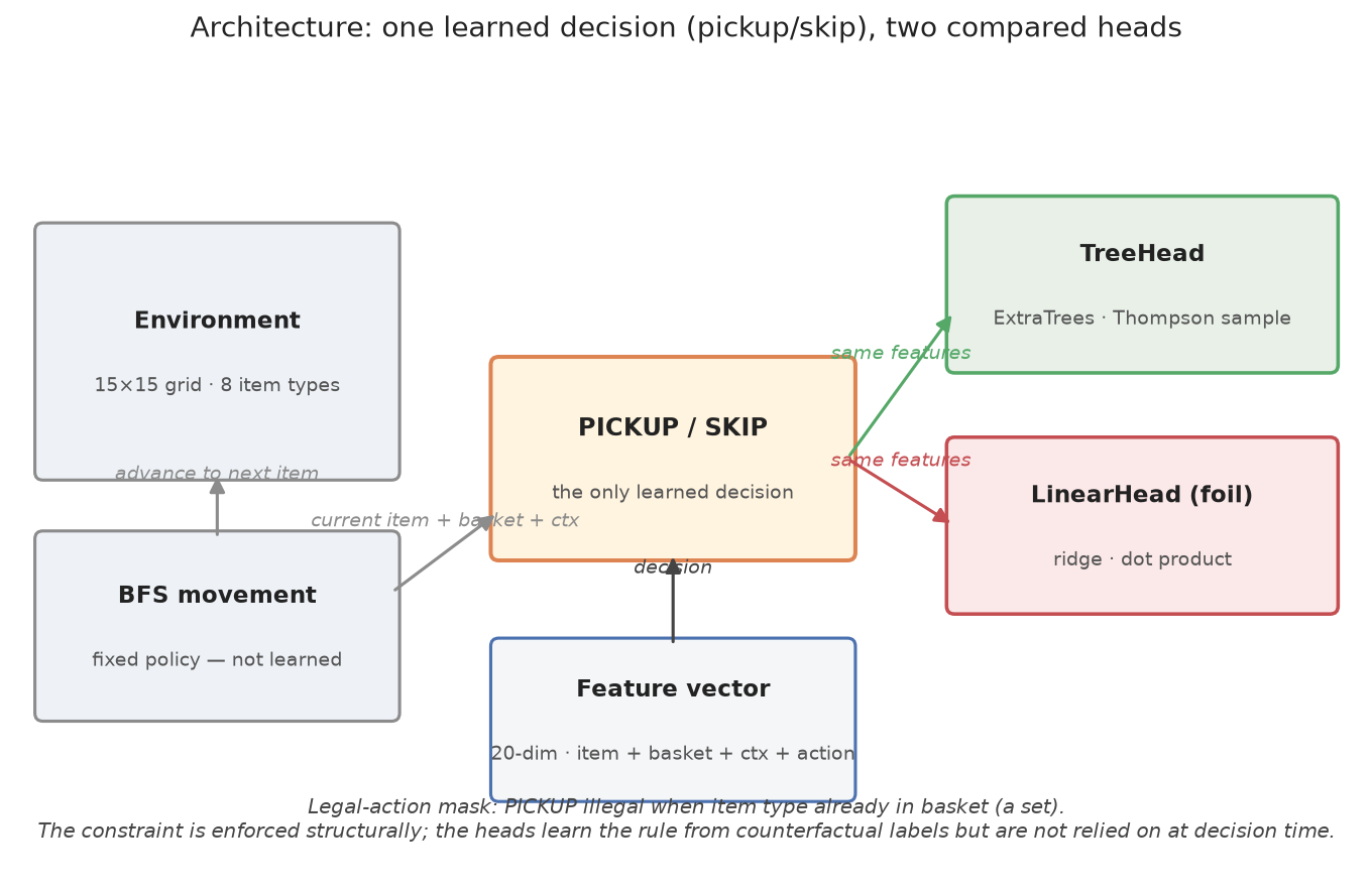
The environment — free BFS movement
Each step the environment presents the next undecided item — the nearest uncollected item by BFS from the agent’s current cell. The agent teleports along the BFS path. Items are never obstacles; movement is deterministic and carries no reward. This is the move that isolates the learned decision: the agent cannot express “I walked past beer but chose not to pick it up” if walking past beer is itself a learned action. By making movement a fixed policy owned by the environment, the only thing the bandit learns is pickup vs skip — which is exactly the “which set of items is compatible in this context” question the regime is about.
The feature vector — 20 dimensions, deliberately raw
Per decision the env emits a 20-dimensional stack, two rows (SKIP, PICKUP), identical except the action one-hot:
[item one-hot, 8]— the encountered item.[basket one-hot, 8]— current basket (captures item×basket interactions).[ctx one-hot, 2]— current time-of-day.[action one-hot, 2]— SKIP or PICKUP.
No pre-computed [item × ctx] columns. Those would let the linear
foil solve the problem by direct lookup and the headline negative
result collapses. The non-linearity has to be discovered by the
function class, not handed to it.
The heads — tree vs linear, identical everything else
Two heads are compared, with identical features, identical data, identical training loops. Only the function class differs.
- TreeHead — an extremely-randomised-trees ensemble (Geurts et al. 2006). Forty trees, each fit on the agent’s accumulated transitions. Across-tree disagreement drives Thompson Sampling: at each decision sample one tree’s prediction per action and act on the sample, so high-disagreement items get explored.
- LinearHead — ridge regression in closed form. Same 20 features, same per-step reward target. The foil. Its dot product has no item×ctx cross term, so it averages each flip item’s value to zero across contexts and treats every flip item as worthless.
The point of the foil is honesty. The question is not “can a model learn this rule” — obviously a model can — but “does the non-linearity actually matter, or could a simpler model have done it?” Running the linear head on the same features as the tree, with the same training data, isolates the function class as the only variable. If the linear head solves the problem, the feature design is too easy and the thesis collapses. If it plateaus at chance while the tree clears 0.84, the non-linearity is load-bearing.
Counterfactual training — both arms, every decision
At each decision the harness knows the reward both arms would have
yielded (skip → 0; pickup → the basket-score delta the item would
cause). It feeds both rows to observe(), so the head sees
balanced 2-arm data and can contrast pickup vs skip directly. This is
the single biggest reason convergence is fast: without it the head
only sees the action it happened to take, and the tree has to infer
the contrast from skewed data over many episodes.
The legal-action mask — constraints are not learned
Picking up an item whose type is already in the basket is impossible
(the basket is a set — the bit is already set). At decision time
PICKUP is masked illegal whenever basket[item]=1. This is a hard
constraint, not a learned preference. The duplicate rule still shows
up in the tree’s weights — counterfactual observe keeps feeding
R_DUPLICATE = −0.5 as the PICKUP row’s label for a duplicate cell,
and the §Validation probe shows the conjunction learned — but the
agent is guaranteed to satisfy the constraint regardless of what the
head happens to predict.
This is the clean separation at the heart of the architecture:
structural constraints belong in the action mask; preferences belong
in the head. An earlier draft of this agent relied on R_DUPLICATE
to teach the agent not to pick up duplicates. The tree’s mean Q
mostly learned the rule, but Thompson sampling one tree per action
flipped borderline cells ~17% of the time; the linear foil violated
it 100% of the time. A duplicate is impossible by construction — the
right tool is a mask, not a penalty the head has to rediscover.
The drift detector — EWMA on prediction error
When the context flips mid-episode, the value of every flip item inverts and the model starts mispredicting immediately. The detector watches that signal directly: an exponentially weighted moving average of on the taken action (Ross et al. 2013, the ECDD variant). Two thresholds — warning at , drift at on the standardised EWMA residual ,
where are the EWMA of the error and squared error. At drift, a short forced-random re-explore window opens (six decisions) and an immediate refit fires. Because every decision in this architecture produces a prediction (both arms are scored), the error stream is dense and clean — exactly what a context flip perturbs.
The negative control matters here. The random arm also sees rewards change at the flip — its per-step rewards are noisy but the distribution shifts. Yet the detector fires zero drifts on random. That is because random’s reward stream has no stable mean to deviate from in the first place; its variance swamps the shift. The detector responds to structured drift — a model that was predicting well and suddenly stops — not to any reward variation.
Validation
The agent runs on a 15×15 grid of food items. Eight items — coffee, beer, eggs, flour, sugar, toast, milk, juice — scatter at random. Four of them flip value with context: coffee and eggs are morning-good at , beer and milk are evening-good at , all in the wrong context. The other four are stable in both. The agent must fill a basket of four item types. The optimum in either context is two correct flip items plus two stables for a score of ; random grabbing averages near zero (two right flips plus two wrong flips cancel).
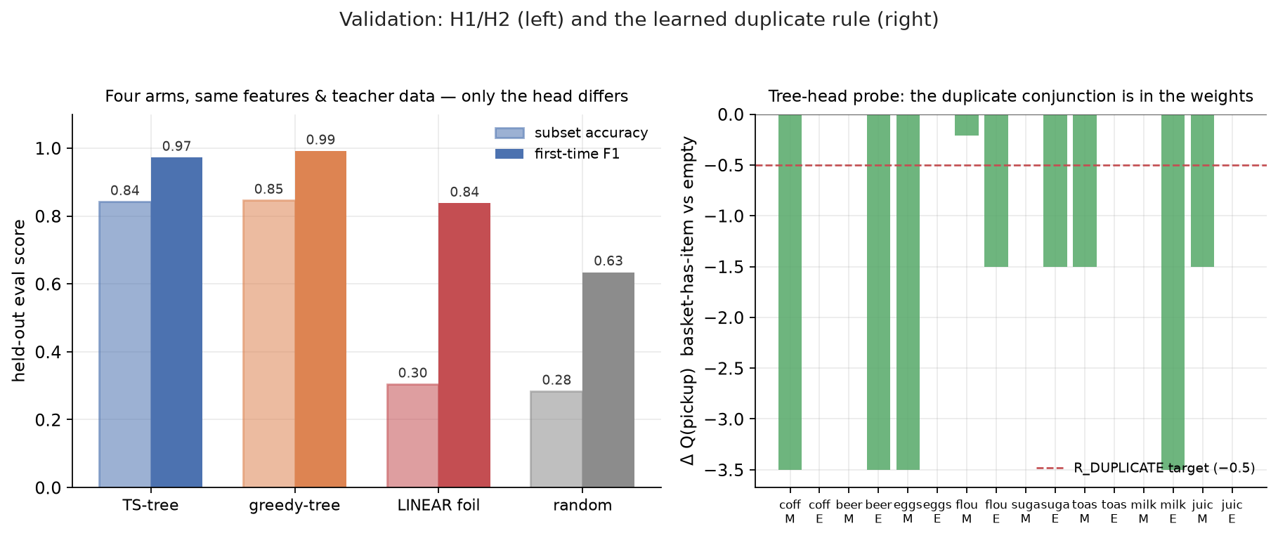
The harness runs four arms — TS-tree, greedy-tree, linear foil, random — across five seeds, on a train/eval split. Each arm gets the same teacher bootstrap (200 counterfactual oracle rollouts seeded into the long-term buffer), then twelve worlds of online training, then twelve held-out worlds of frozen evaluation. Every number below is from the frozen eval phase — does the learned rule discriminate correctly on fresh worlds?
The interaction-term headline (H1, H2)
| Arm | Subset accuracy | First-time F1 | Ratio to TS-tree |
|---|---|---|---|
| TS-tree | 0.84 | 0.97 | — |
| greedy-tree | 0.85 | 0.99 | 1.00× |
| LINEAR foil | 0.30 | 0.84 | 0.36× |
| random | 0.28 | 0.63 | 0.33× |
On held-out eval, TS-tree beats the linear foil by 2.8× on subset accuracy and beats random by 3.0×. The foil sits at 0.30 — essentially at the random baseline — because it cannot represent the item×context conjunction. The tree clears 0.84.
The greedy-tree arm matching TS-tree is the honest result that the non-linearity is in the function class, not in the exploration strategy. Switching from Thompson Sampling to greedy within the tree arm barely moves the number — both can represent the rule. Switching from tree to linear collapses it. That collapse, on identical features and identical data, is the load-bearing finding.
Why two metrics. Subset accuracy (achieved basket score ÷ optimum) is the H1 gate because wrong-context flip items compound penalties — the foil’s indiscriminate pickups actively tank its basket score. But subset accuracy is end-of-episode; it does not grade every decision. First-time F1 grades each pickup/skip call against the optimal action, excluding duplicate encounters (which are forced-skip by the mask and would otherwise pad the score). It also uses F1 rather than accuracy so that an arm which picks up everything (the linear foil, recall 1.0) doesn’t score well on recall alone — it pays in precision for the wrong-context flip items it picks up.
The foil — why linear plateaus
The foil’s failure is structural, not a tuning problem. The ridge solution assigns each feature a single weight. For the item-coffee feature, that weight is the average reward of coffee across all observed transitions — morning transitions where coffee gave and evening transitions where it gave . The average is zero. So the linear model’s prediction for picking up coffee is the same in both contexts: approximately zero. It treats every flip item as worthless and, because pickup and skip look identical to it, defaults to skip. Its 0.30 subset accuracy comes from occasionally picking up stable items by chance, not from any learned discrimination.
The tree does not average. It splits on item-coffee, then below that
splits on ctx-morning, producing a leaf that holds and another
that holds . Two splits and the rule is exact. The non-linearity
is not a deficiency of the linear model that more data could fix; it
is a provable property of the dot product. No amount of training data
closes that gap.
Drift on a mid-episode context flip (H3)
Each flip-schedule episode starts in the morning and flips to evening at decision 25. Coffee goes from to immediately. The EWMA detector fires eight drifts across five seeds (and zero on the random arm, which has no structured reward stream to drift). The post-flip pickup pattern on the flip items inverts — coffee goes from picked-up to skipped; beer the opposite — within the forced re-explore window that follows each drift event. Fast enough to relearn the rule while the post-flip world is still fresh.
Pre-train carryover (H4)
The teacher bootstrap (200 counterfactual oracle rollouts seeded into the long-term buffer) gives a +0.33 first-episode accuracy delta over cold start (1.00 pretrained vs 0.67 cold). The pre-trained agent acts on its model from step one; the cold-start agent spends the first episode in random exploration. The two-timescale memory means the teacher’s transitions persist across the whole run — the long-term buffer is never reset, only capped at 800 rows.
The constraint regression check
Across every arm and every eval world, the duplicate-pickup rate is 0.000. This is not a quality metric; it is a regression check on the legal-action mask. The linear foil, which would violate the constraint 100% of the time without the mask, picks up zero duplicates. The mask is doing the work; the heads are doing the learning; the metrics verify both.
Constraint and learning are separate questions
The cleanest way to see why the mask and the head belong in different places is to ask what goes wrong if you collapse them.
Collapse the mask into the head. Drop the legal-action constraint
and rely on the R_DUPLICATE penalty to teach “skip duplicates.” The
tree’s mean Q mostly learns the rule (the §Validation probe shows
on the relevant cells), but Thompson sampling draws one tree
per action — a single over-optimistic tree resurrects PICKUP on a
borderline cell and the agent picks up a duplicate 17% of the time.
The linear foil violates 100% of the time because its dot product has
no basket[item] × action term. Both failures trace to the same
cause: asking the function class to enforce a structural property it
cannot represent reliably. The mask answers “can the agent violate
the rule?” (no, always). The head answers “could the model represent
the rule?” (yes for the tree, no for the linear foil). Conflating them
turns a guaranteed property into a probabilistic one.
The other direction — enforcing preferences in the mask — is just encoding the policy by hand. You could hard-code “skip coffee in the evening” as a mask rule. But then you have not built an agent; you have built a lookup table. The mask is for constraints the environment guarantees (the basket is a set); the head is for preferences the agent must learn (coffee is morning-good). Crossing that line in either direction breaks something.
This is the architectural point of the post, and it generalises past the kitchen. Anywhere the action set has structural constraints (capacity limits, type uniqueness, mutual exclusivity, scheduling deadlocks), those constraints belong in the mask — not as penalty terms the learner has to rediscover, and not as hand-coded policy rules that bypass learning entirely.
Where this pattern actually lives
The regime maps onto a long list of deployed problems where the value of a choice depends on what else has been chosen or on external context.
Recommendation bundles
A streaming service selecting a session’s content mix. Each item has a standalone value, but the bundle’s value is non-additive: two thrillers back-to-back fatigue the viewer; a documentary pairs well with a related drama. The “context” is time-of-day or session intent (evening entertainment vs morning news). A linear ranker cannot represent “this item is good in this slot type given what is already in the session.”
Configuration and feature selection
A system assembling a configuration from many toggles. Some toggles are individually beneficial but conflict (two caching strategies that double-cache). The value of enabling A depends on whether B is enabled. The “context” is workload (A is good under read-heavy, bad under write-heavy). A linear model over toggle indicators misses the conflicts.
Basket and portfolio construction
Any setting where the agent assembles a subset under a cardinality constraint and the subset’s value is non-additive. Investment portfolios (hedge correlations), meal planning (nutritional balance), shopping baskets (promotional cross-discounts). The context — risk regime, dietary target, promotional period — flips the value of individual items.
Adaptive UI composition
A dashboard selecting which widgets to show. Each widget has a standalone utility, but two widgets showing the same metric in different forms conflict; the value of one depends on whether the other is present. The “context” is the user’s task, which shifts through the day.
When it fails
Do not use it when items do not interact — if the reward really is additive over individual items, a linear value head is simpler, faster, and exactly correct, and the tree is overkill. The linear foil in this post scores 0.30 only because the regime is non-additive by construction; in an additive regime, it would win.
Do not use it when the interaction structure is too rich for axis-aligned splits. If the rule depends on a continuous combination of many features (a deep XOR across four dimensions, say), even a deep tree struggles, and a neural bandit with a Bayesian last layer becomes the better trade. This post’s regime is specifically the one where the interactions are low-order conjunctions (item AND context) that two or three splits can enumerate. That is a large and useful class — most real “compatibility” rules are pairwise or triple — but it is not all of them.
The cleanest tell that you are in this regime: the same item has different values in different contexts, and a linear model’s per-item weights cannot track the difference. If you fit a linear regressor on the logged reward and it consistently underperforms a tree on the same features, you are seeing the conjunction gap. That gap is the load-bearing finding of this post.
Conclusion
The predecessor post ended by punting on non-linear interactions: at that scale, it said, a neural bandit becomes the better trade. This post is the punt taken back, and the finding is that the punt was premature. Non-linear does not mean neural. It means interaction-aware. And the cheapest interaction-aware function class available — a tree ensemble — handles exactly the regime where a linear bandit gives up: low-order conjunctions of features that two or three splits can represent exactly.
The two architectural moves that make this tractable are each a response to a concrete failure mode.
- Counterfactual both-arm training gives the head balanced 2-arm data every decision. Without it the tree infers the pickup-vs-skip contrast from skewed data over many episodes; with it, the rule converges in a couple of episodes.
- The legal-action mask enforces structural constraints structurally. An earlier draft relied on a reward penalty to teach “skip duplicates”; Thompson sampling violated it 17% of the time and the linear foil 100%. The mask makes the constraint a guarantee; the head’s learned conjunction is evidence about the function class, not a guardrail.
- The linear foil on identical features is the honesty ledger. The point of this post is not “a model learned a rule.” It is “the rule is non-linear, and here is the linear model that provably cannot learn it on the same data.”
The feature design and the mask are general machinery — they would carry over to a neural bandit unchanged. The head is where the function-class question lives, and the answer in this regime is: trees. Not because they are fashionable, but because their axis-aligned recursive partitioning is exactly the representation that low-order feature conjunctions ask for. When the conjunctions get deeper than the tree can handle, the same architecture swaps in a neural last layer without touching the feature design or the mask. That is the next post.
References
- Geurts, P., Ernst, D. & Wehenkel, L. Extremely Randomized Trees. (Machine Learning 63(1)–42, 2006) — the splitting rule the tree head uses; one random threshold per feature, variance reduction by averaging.
- Read, J., Pfahringer, B., Holmes, G. & Frank, E. Classifier
Chains for Multi-label Classification. (ECML PKDD 2009, LNCS 5781)
— captures label interactions by passing earlier-label predictions
as features. The
[basket]feature block is the same idea, made sequential. - Chen, W., Wang, Y. & Yuan, Y. Combinatorial Multi-Armed Bandit: General Framework and Applications. (ICML 2013) — regret bounds for non-additive set reward. The kitchen grid is the small- regime where the offline oracle CUCB needs is trivial.
- Chen, W., Wang, Y., Wang, L. & Li, J. Combinatorial Multi-Armed Bandit with General Reward Functions. (NeurIPS 2016) — extends to arbitrary non-linear reward under bounded smoothness.
- Rhuggenaath, J., Akcay, A., Zhang, Y. & Kaymak, U. Algorithms for Slate Bandits with Non-Separable Reward Functions. (arXiv.09957, 2020) — directly studies the case where slate reward cannot decompose as a sum over slots. The canonical citation for “reward of a set is non-additive.”
- Ross, G. J., Adams, N. M., Tasoulis, D. K. & Hand, D. J. Exponentially Weighted Moving Average Charts for Detecting Concept Drift. (Pattern Recognition Letters 33(2)–198, 2013; arXiv.6018) — the EWMA-ECDD detector. Continuous-signal drift detection on a streaming error rate.
- Riquelme, C., Tucker, G. & Snoek, J. Deep Bayesian Bandits Showdown. (ICML 2018) — the Neural Linear recipe (frozen embedding → Bayesian last layer), which is the principled next step when the conjunctions get too deep for tree splits.
- Osband, I., Blundell, C., Pritzel, A. & Van Roy, B. Deep Exploration via Bootstrapped DQN. (NeurIPS 2016) — ensemble as approximate posterior. The TS-tree head’s across-tree sampling is the same idea in the bandit setting.