MoB Queen: Mixture of Bandits with a Global Density Map and a Queen Move
Assets & Materials doi: 10.5281/zenodo.21471737
| Mixture of Bandits — Interactive simulation, MoB Global variant. The same planner with a queen-jump action; toggle between baseline, gated, and global from the panel. | https://blog.vski.ai/mob/?model=mob_global |
| MoB: Mixture of Bandits. (Predecessor, v2) | https://blog.vski.ai/posts/mixture-of-bandits/ |
| The Sequential Recommender: Fitted Q-Iteration. (v1) | https://blog.vski.ai/posts/sequential-recommender/ |
This essay is third in a line of work on the Mixture of Bandits (MoB) architecture — a stateless agent that discovers reward in a world it cannot see, using a noisy local sensor and one linear value function shared across every world it will ever meet. The original MoB design added a six-weight logistic gate that learned to disable the planner’s long leap in exactly the states where that leap walked past a cluster it could have collected — a per-state action mask, not a second expert. The gain showed up exactly where it was aimed: clustered worlds. The lesson was that the planner was not lacking a capability; it was making a specific, repeatable mistake on a specific, identifiable class of states, and the right fix was to learn to detect that class of states and forbid the action that was wrong there.
This essay adds one more move to the same architecture — a queen jump aimed at the highest-density cell the agent believes is still out there — and shows that the same recipe generalises to the failure mode v2 could not touch: sparse worlds where the action set itself is too short to escape the visited footprint.
The Gold Digger
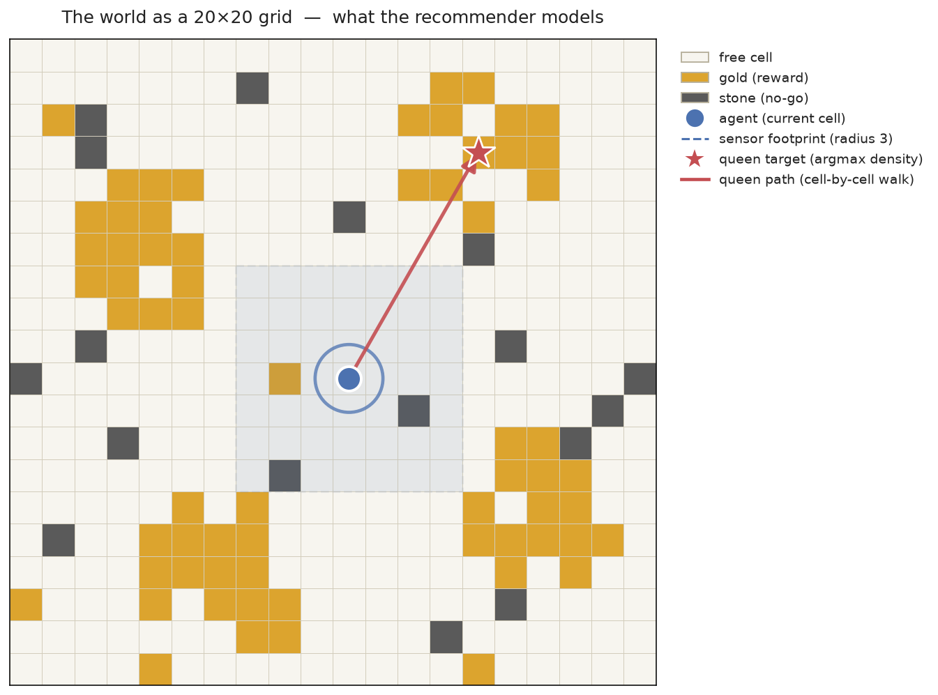
We work inside a concrete running model that we call Gold Digger. It is a recommender engine stripped down to its load-bearing geometry: an agent on a grid, reward painted on some cells, obstacles on others, a sensor that sees only what is near. The grid is the cleanest place to study the architecture because every quantity we care about — exploration, exploitation, bypass, density, frontier — has a literal spatial meaning. The agent’s job is to collect as much gold as it can before its step budget runs out.
The grid is a state space, not a map. Each cell is a candidate item: a song in a catalogue, a product in a store, a configuration of a tunable system, a region of a search space. Gold is reward — a click, a conversion, a successful probe. Stones are no-gos — items the user will not engage with, configurations that violate constraints, regions known to be empty. The agent’s position is its current context: what it has just shown, tried, or measured. A move is the next recommendation, the next experiment, the next query. The sensor is whatever local feedback loop the deployment gives you — dwell time on the last few items, residuals on the last few fits, telemetry from the last few probes. Everything outside the sensor footprint is inferred, one noisy observation at a time, into a Bayesian belief map. That belief map is the recommender’s user model.
The regime
The agent operates under four constraints that together define the low-cost sequential exploration regime: it is stateless across episodes (every episode starts with a flat belief map; what persists is the learned Q-function, not memory of yesterday’s world, so it must generalise across worlds it has never seen); it has a noisy local sensor (outside a small radius it knows nothing and has to infer everything into the belief one tick at a time); moves are cheap (a length-1 hop and a length-8 leap cost the same — one planner step — so the binding resource is the step budget, not motion); and the world is stochastic (reward layouts are redrawn every episode, so the agent cannot hard-code a strategy and has to infer where reward is from belief). Two shortcuts fall out of those constraints and are off the table by construction: a cluster-detecting sensor would be cheating (it is the ground-truth side-channel the agent is supposed to be inferring), and a hand-coded strategy would not be ML (the question is whether the policy can be learned, not whether a human can hand-write it). The agent’s job, inside all four constraints, is to maximise collected reward before its step budget runs out.
What the previous generations could not do
The first generation learned to move toward belief: a single linear Q-function over the path features, smooth policy, beats random by 1.21–1.66× depending on world type. On clustered worlds it developed a specific, repeatable failure — the longest leap would grab a sliver of a dense patch and sail past the rest of it.
The second generation fixed that by gating the long leap and adding a short orthogonal knight action. A six-weight logistic regression, trained on labelled bypass events, learned to detect the specific states where a long leap would walk past a cluster it could have collected — and to forbid that leap in exactly those states, forcing a re-pick from the short-hop menu. The gain showed up exactly where it was aimed: +7% on clustered worlds.
Both generations shared one assumption: the agent would eventually find a cluster, and the question was what to do once it had. On sparse worlds that assumption is half-right. There is no cluster, but there is still reward, scattered thin, across a map the agent cannot see and cannot memorise. v1 and v2 both beat random on those worlds — 1.66× and 1.91× respectively — but they leave a specific failure on the table, and it is not the failure the gate was built to fix.
What happens on sparse worlds is mechanical. The agent’s belief map
converges — slowly, then suddenly — to a picture where every visited
cell has low bGold (because the gold there was collected) and every
unvisited cell has prior bGold (because the agent has not learned
otherwise). The correct move, given that picture, is to leap toward
unvisited space. The planner does leap. But the planner’s longest leap
is short — four cells, in the deployed action set — and unvisited space
is often further than that: across the visited footprint, on the other
side of where the agent has been spending its time. The agent takes its
longest leap in the right direction, lands still inside its visited
footprint, re-observes cells it has already emptied, and repeats. It
is not wandering randomly — its policy still beats random by 1.91× —
but it is circling relative to its own potential, because the action
set does not contain a move long enough to escape the visited footprint
in one step.
The second generation’s gate is no help here, by design. The gate’s
signal is local_minus_global — the regime signal that fires when
local belief exceeds global belief. On a sparse world, everywhere is
equally empty. The signal is flat. The gate does not fire. The knight
action does not help either — its two-and-one hop is shorter than the
length-4 leap, not longer. The circling-on-sparse-worlds failure is a
new failure mode, addressable only by a new action whose reach
exceeds the longest leap.
The feature space
The agent does not see pixels. It sees eleven engineered features per candidate action, computed from the belief map at decision time. The same eleven features describe every action; what differs is the action itself — direction, length, and (now) kind.
The encoding trick is that a candidate action defines a path through the grid, and the path is what gets summarised. For a length- leap in direction , the path is the cells from the agent’s current position along . The features aggregate belief along that path:
| # | Feature | What it captures |
|---|---|---|
| 0 | dest_bGold | bGold at the destination cell — is the landing spot promising? |
| 1 | dest_bStone | bStone at the destination — does the path end in an obstacle? |
| 2 | path_gold_sum | Sum of bGold along the path — expected gold on the trajectory |
| 3 | path_clear | 1 if every cell on the path is walkable, 0 otherwise — the mask |
| 4 | local_minus_global | Local mean bGold − global mean — the regime signal |
| 5 | dest_recency | Recency of last visit to the destination — am I going back? |
| 6 | length | Leap length, normalised — how far am I committing? |
| 7 | dest_unvisited | 1 if destination unvisited, 0 otherwise — new ground signal |
| 8 | dir_dx | Direction’s x-component — encodes direction as two features |
| 9 | dir_dy | Direction’s y-component — so the linear Q can score each direction smoothly |
| 10 | bias | Constant 1 — the intercept |
The encoding is general. Anything that can be framed as a path through a state space, with local evidence along it, fits.
The belief map itself is a (bGold, bStone) posterior field, updated
tick by tick from the noisy sensor. Cells inside the latest sensor
footprint are sharp; cells outside decay toward a soft prior. There is
no second map, no global view, no learned forecaster. There is just
the belief, masked by what has been visited, read at the right time.
The queen jump
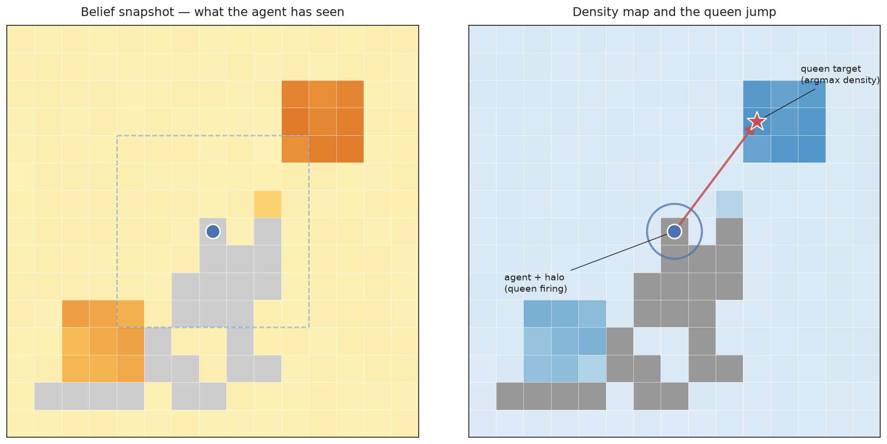
The third generation adds one new action: a queen move, in honour of the chess piece that moves any number of squares in any direction. Eight new candidate actions — one per direction — are appended to the planner’s menu. Each queen action means: jump along this direction, as far as the density map says is worth jumping, walking cell by cell and collecting reward on the path.
Three pieces make this work, and all three are regime-faithful.
The density map
The density map is the belief map, read differently:
where is a frontier bonus — 1 if the cell is on the boundary between visited and unvisited space (more than half of its 3×3 neighbourhood unvisited), 0 otherwise — and is a fixed weight.
It is the Yamauchi (1997) frontier-based exploration formula in two lines, applied to a belief map the agent already maintains. The mask zeros out every cell the agent has already explored — so the density map literally cannot point the agent back where it has been. The frontier bonus tilts the map toward the boundary of the known, because that is where each new step exposes the most new sensor footprint.
The top-1 precision of this map — of the argmax density cell, how often is it actually gold? — is roughly 1.5× to 2× the uniform gold fraction on sparse worlds. That is enough signal to aim a jump. It is not enough signal to aim a short hop, which is why the queen is a long jump: the per-cell probability of reward is low, but the path walks enough cells that the expected collected reward exceeds any short-hop alternative.
The queen target
For each of the eight directions, the agent scans the density map in a
forward cone along that direction and picks the argmax-density cell
whose straight-line path from the agent’s current position is walkable
(no stones, in bounds). If no such cell exists in that direction — the
direction is blocked, or every unvisited cell in the cone is on the
wrong side of an obstacle — the queen action gets path_clear = 0 and
is masked out of the argmax. The queen action is physically possible
or it is not on the menu.
The walk itself is cell-by-cell, exactly like the existing leap. Per-cell reward (gold collected, stone bumps, recency decay) is applied along the path; the agent simply moves further per planner step than a length-8 leap allows. The planner still consumes one step per queen action — the same budget as a length-1 hop or a length-8 leap. The queen is not free; it is cheap in the same currency as everything else.
The planner learns when to use it
Here is the design choice that keeps the queen from being a degenerate
“always jump” rule: the eight queen actions use the same eleven
features as the leaps. They are appended to the action set at indices
32–39, and the planner’s linear Q-function scores them with the same
weights it uses for everything else. The features aggregate over the
queen path: dest_bGold is the density at the queen target,
path_gold_sum is the sum along the walk, length is the Chebyshev
distance to the target.
The planner learns the rest. When local reward is dense — a cluster,
the gate’s regime — path_gold_sum for a length-2 leap inside the
cluster beats the queen’s longer-but-thinner path, and the planner
picks the leap. When local reward is sparse and the agent has been
circling, dest_unvisited and the density signal push the queen’s
score above any local leap, and the planner picks the queen. The
when is learned; the where comes from the density map; the how
far comes from the walk.
This is deliberately not a separate gate. The second generation used a logistic gate because the choice it had to make was binary — allow length-8, or disallow it. The third generation’s choice is not binary: it is which of eight queen directions, versus any of twenty-four leaps, in this state. That is exactly what a Q-function does. Adding a gate on top would be adding a classifier to decide when to ask the classifier you already have.
The solid green box is unchanged from generation one: the same linear Q-function, the same eleven features, the same closed-form fit. The solid blue box is new but tiny — it is the density formula above, a few lines of code, no learned weights. There is no second value function. There is no gate. There is just a new action whose aim comes from the belief the agent already maintains.
Results
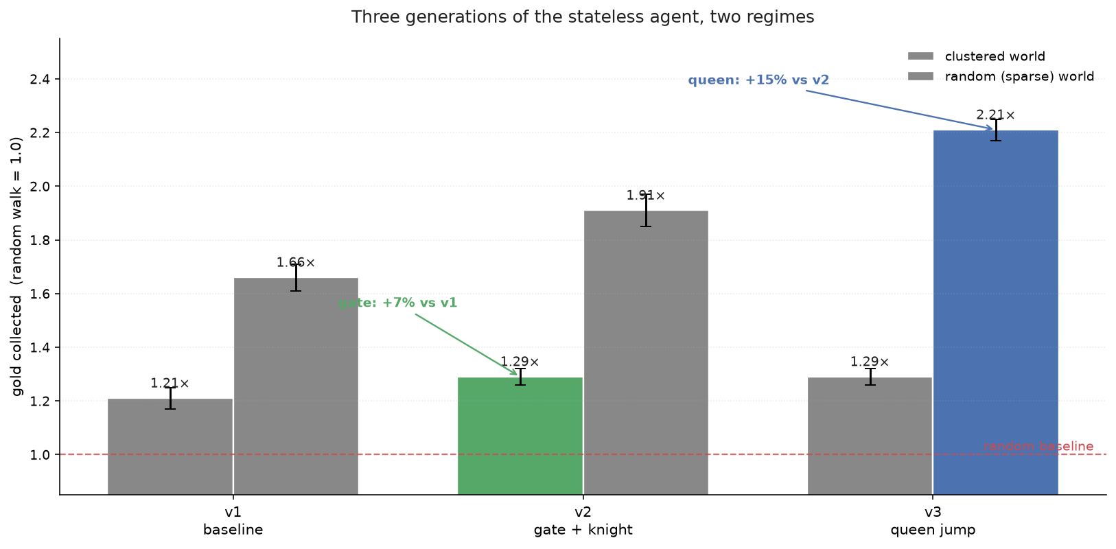
Three generations, two regimes, one matched-pair evaluation protocol. For each (world-seed, train-seed), train the planner on a mixed-world distribution, fit any gates or queen paths, and evaluate twelve episodes per arm with the same world layouts snapshotted across arms. Random baseline is the same protocol with the planner’s weights frozen at initialisation.
| Model | Clustered world | Random (sparse) world | Marginal gain |
|---|---|---|---|
| v1 — baseline planner | 1.21× random | 1.66× random | (baseline) |
| v2 — + bypass gate + knight | 1.29× random | 1.91× random | +7% clustered, +15% random |
| v3 — + queen jump | 1.29× random | 2.21× random | +0% clustered, +15% random |
Numbers are means over 3 training seeds × 12 matched-pair eval episodes per arm, on 15×15 worlds with a 150-step budget. Source: the research notebook, Phase 4 four-arm A/B isolation.
Two things to read off the table, and both are the point.
No generation dominates. Each one wins in the regime it was
designed for and ships at zero cost to the regimes that already
worked. The v2 gate is silent on sparse worlds because
local_minus_global is flat there — there is no cluster boundary to
detect — and it ships its clustered-world gain anyway. The v3 queen is
silent on clustered worlds because, on clustered worlds, v2 already
collects every gold cell the agent’s sensor can see; there is nothing
left for a longer jump to find. The queen’s learned-when mechanism —
the planner simply picking the queen action only when its Q-value beats
the leaps — keeps the queen out of states where short hops pay better.
Each generation’s marginal gain is in a different regime. v2 added 7% on clustered worlds (the gate’s target) and 15% on random worlds (the knight’s orthogonal-hop target — the knight helps everywhere, the gate helps only where it fires). v3 added 0% on clustered and 15% on random. The clustered column saturates at v2 because the agent already collects ~100% of visible gold there; the random column climbs every generation because each one added a tool for finding gold that the previous one lacked. The story is not “each model is strictly better” — v3 is exactly v2 on clustered worlds. The story is each model opens a regime the previous one could not reach, without losing anything it already had.
The queen’s +15% on sparse worlds is the cleanest signal in the table, and the 4-arm A/B isolation in the notebook breaks it down. A queen action aimed at a random target — same action, same learned-when, no density map — collects 0.54× baseline gold: catastrophic, because jumping long distances to nowhere is worse than not jumping. The same queen action aimed at the density map collects 1.15×. The density map is the whole signal; the learned-when is just the gatekeeper. This is the regime’s answer to “is the density map doing the work, or is the queen action doing the work?” — the density map. Strip it out and the queen is actively harmful.
Where this pattern actually lives
The grid is a clean place to see the recipe work. The recipe is not about the grid. Low-cost sequential exploration is a broad regime, and the queen move — a long, aimable jump toward inferred-dense unvisited state space — has direct analogues in any domain that satisfies its two assumptions: moving is cheap, and the agent maintains a belief over where reward might be.
Probing and signalling
The literal case. A laser shot, a sensor ping, a satellite tasking, a network probe — all cost the action, not the distance. Firing a laser one metre and firing it one kilometre cost the same number of planner steps. The agent’s budget is shots fired, not ground covered. On any problem of that shape, the queen move is the right primitive: aim the shot at the highest-density unobserved cell in the belief, not at the nearest unobserved cell. Frontier-based robotics exploration (Yamauchi 1997) has used exactly this for three decades. The MoB Queen’s contribution is to show that the same primitive fits inside a learned value function — the agent learns when frontier-jumping beats local search, instead of always doing it.
Adaptive recommendation
A recommender that adapts fast and does not tire the user is a low-cost sequential explorer. Each item shown is a move; the user’s response is a noisy local observation; the recommender maintains a belief over what the user wants. The catch is that every move the recommender makes is also a small cost to the user’s attention — exhaust the budget and the user leaves.
A pure short-hop recommender (show one more item like the last) circles in the user’s stated preferences forever, never finding the long-tail interest that would surprise them. A pure long-leap recommender (maximise diversity) jumps around the catalogue so aggressively that it never builds a coherent session. The queen move is the middle path: stay local when local is working, jump toward unexplored high-density regions of the catalogue when local is circling. That is, structurally, what good session-based recommendation already does — the MoB Queen is the formal version, with the when learned by a value function and the where aimed by a density read of the user model. Production sequential-RL recommenders (Chen et al. KDD 2019, McInerney et al. 2023) handle the same tension with full sequential RL; the queen move is the cheaper, convex-where-possible version for teams that cannot afford to ship a divergent value function.
AI personalisation — meta-parameter selection
The fastest-growing analogue. A modern agent — LLM-driven, tool-using, configurable — has dozens of meta-parameters: temperature, retrieval depth, tool subset, prompt template, model selection. Picking them per-query is a bandit problem. Picking them across a session, where each choice both delivers reward (task success) and changes what the next query should do (context drift), is a sequential bandit.
The queen move fits cleanly. The belief map is what meta-parameter combinations have worked for which kinds of queries; the visited mask is what has been tried enough times; the density map is which untried combinations are most likely to pay off, given what has worked so far. A short hop is tweak the temperature by 0.1; a queen jump is switch retrieval off and tool-use on for this query type, because the density of untried-but-promising configurations sits there. The random component the regime demands is what keeps the personaliser from overfitting to one user’s history — it stays exploratory enough to recover from a bad early impression.
Sequential A/B testing
A/B testing infrastructure that lets you adapt mid-experiment — multi-armed bandits at the cell level — is a low-cost sequential explorer. Each arm pull is cheap; each pull both delivers reward (measured lift) and sharpens the belief about which arm is best. The budget is total exposures, which is bounded by traffic. The queen move is allocate the next chunk of traffic to the arm whose upper-confidence-bound is highest among under-explored arms — which is structurally what UCB and Thompson sampling already do, but formulated as a single aimable jump in belief space rather than a per-arm allocation rule.
Conclusion
Three generations of one agent. The first learned to move toward belief. The second learned to stay inside a cluster by gating the long leap in states where it bypassed dense reward. The third learns to escape its own footprint by jumping toward the highest-density unvisited cell the belief can identify. Each generation added one piece — a value function, then a classifier, then a new action fed by a density read of the existing belief — and each piece won in its own regime without breaking what came before.
The pattern across the three is the actual lesson. The disease was never the agent lacks a capability. The disease was always a specific class of states where the current action set could not express the right move. On clustered worlds, the right move was already in the action set (length-2 leaps) but the planner kept picking the wrong one (length-8) — so the fix was to mask the wrong one. On sparse worlds, the right move was not in the action set at all — no length of leap was long enough to escape the visited footprint — so the fix was to add a longer move, aimed by the belief. Diagnose the failure mode first. If the right action exists but is not being chosen, restrict the menu. If the right action does not exist, add it, and let the planner learn when to use it.
References
- Sutton, R. S. & Barto, A. G. Reinforcement Learning: An Introduction, 2nd ed., MIT Press, 2018 — Ch. 2 (bandits), §2.9 (associative search), Ch. 3 (finite MDPs). Full PDF.
- Yamauchi, B. A Frontier-Based Approach for Autonomous Exploration. (IEEE ISRE 1997) — the frontier-based exploration formula the density map uses. A 1997 paper that still describes how most exploration robots decide where to go next.
- Ernst, D., Geurts, P. & Wehenkel, L. Tree-Based Batch Mode Reinforcement Learning. (JMLR 2005) — Fitted Q-Iteration, the planner’s training algorithm. Three generations in, still the same closed-form fit.
- Munos, R. & Szepesvári, C. Finite-Time Bounds for Fitted Value Iteration. (JMLR 2008) — the convergence guarantee that lets the planner stay linear and still be safe to deploy.
- Auer, P., Cesa-Bianchi, N. & Fischer, P. Finite-time Analysis of the Multiarmed Bandit Problem. (Mach. Learn. 2002) — UCB, the algorithm the queen move echoes in belief space: aim at the highest-density under-explored cell.
- Chen, M. et al. Top-K Off-Policy Correction for a REINFORCE Recommender System. (KDD 2019) — production YouTube RL recommender; the long-horizon side of session-based recommendation at scale.
- McInerney, J. et al. Optimizing Audio Recommendations for the Long-Term. (2023) — production Spotify RL over podcast listening journeys; the same explore-exploit tension in a deployed recommender.
- Russo, D. & Van Roy, B. Learning to Optimize via Posterior Sampling. (MOR 2014) — Thompson sampling as a principled exploration policy; the queen move’s aim at inferred density is the deterministic analogue.
- Executable companion. Mixture of Bandits demo — MoB Global variant — the live agent with the queen jump enabled. Toggle between baseline, gated, and global from the panel and watch which regime each one wins in.