Primer to Gradient Descent

Gradient descent is the most widely used optimisation algorithm in machine learning, and the idea behind it is surprisingly simple. This essay is the preface for what comes next: without understanding gradient descent, you will not understand the majority of machine learning. So before we get to bandits, recommenders, or neural networks, we will build the one idea they all rely on — the notion of a slope, and of stepping downhill along it.

The throughline is the derivative. Regression measures an average slope. Differentiation makes that slope instantaneous. Partial derivatives extend it to many variables. Gradient descent puts all three to work to learn.

Gradient descent in one analogy

If you were five years old, here is how I would explain it. Imagine you are adjusting the volume on your TV. Too loud and the neighbours complain; too low and you cannot hear the show. Somewhere in between there is a volume that is just right.

Now assign names to the pieces, because those names are the whole of machine learning in miniature. The change in volume as you twist the knob — how much louder or quieter it gets per click — is the derivative. The volume difference itself is $\Delta$ (capital delta, “change in”), and the rate at which loudness changes per click is the slope: $\text{slope} = \Delta y / \Delta x$. The act of twisting the knob and measuring what happens is differentiation.

The signal you get back from the world — a knock on the wall from the neighbours, or straining to hear a whisper on screen — is the error. The closer you are to the perfect volume, the smaller the error. Repeatedly measuring that error and nudging the knob in the direction that shrinks it, a little at a time, until no one complains — that process is gradient descent.

Formally, gradient descent minimises a cost function $J(\theta)$ by updating the parameters in the direction of the negative gradient:

$$\theta_{t+1} = \theta_t - \eta \, \nabla J(\theta_t)$$

Here $\theta$ is the knob (the model’s parameters), $\eta$ is the learning rate (the size of each nudge), and $\nabla J$ is the gradient — the slope of the error, pointing uphill. We subtract it precisely because we want to go down. The four sections below build this one rule up piece by piece, and each has an interactive counterpart you can play with.

Open the interactive demo

Linear regression

Start with the simplest possible question: given two points, what is the trend between them? Take $(1, 10)$ and $(10, 1)$. Regression finds the average rate of change between them — a single straight line that captures the macro-level trend:

$$\text{slope} = \frac{\Delta y}{\Delta x} = \frac{1 - 10}{10 - 1} = -1$$

On average, for every one step to the right we drop one step down. That number, $-1$, is the slope of the line of best fit. It is “best” in a specific, narrow sense: it minimises the total squared distance between the line and the points. We will return to that “minimises” word — it is where gradient descent lives.

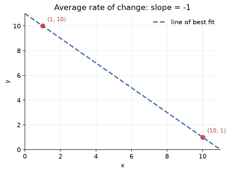
The slope here is an average — it pretends the world changes at a constant rate everywhere between the two points. Reality is rarely that obliging. The line is a summary, not the truth; useful, but blunt. To get sharper we need to stop averaging over an interval and start asking what is happening at a single point.

Open the interactive demo — Section 1

Differentiation

A derivative is just a regression line where the two points are infinitely close together. Take the curve $f(x) = x^2$ and fix a point on it, $A$, at $x = 2$ (so $y = 4$). Place a second point $B$ a distance $\Delta x$ to the right, and draw the line through $A$ and $B$. That line is the secant, and its slope is the average rate of change between the two points — exactly the regression slope from the previous section.

Now slide $B$ toward $A$. As $\Delta x$ shrinks from $4$ to $1$ to $0.1$, the secant line pivots and settles. In the limit, when $B$ sits essentially on top of $A$, the secant becomes the tangent — the instantaneous rate of change, which is the derivative.

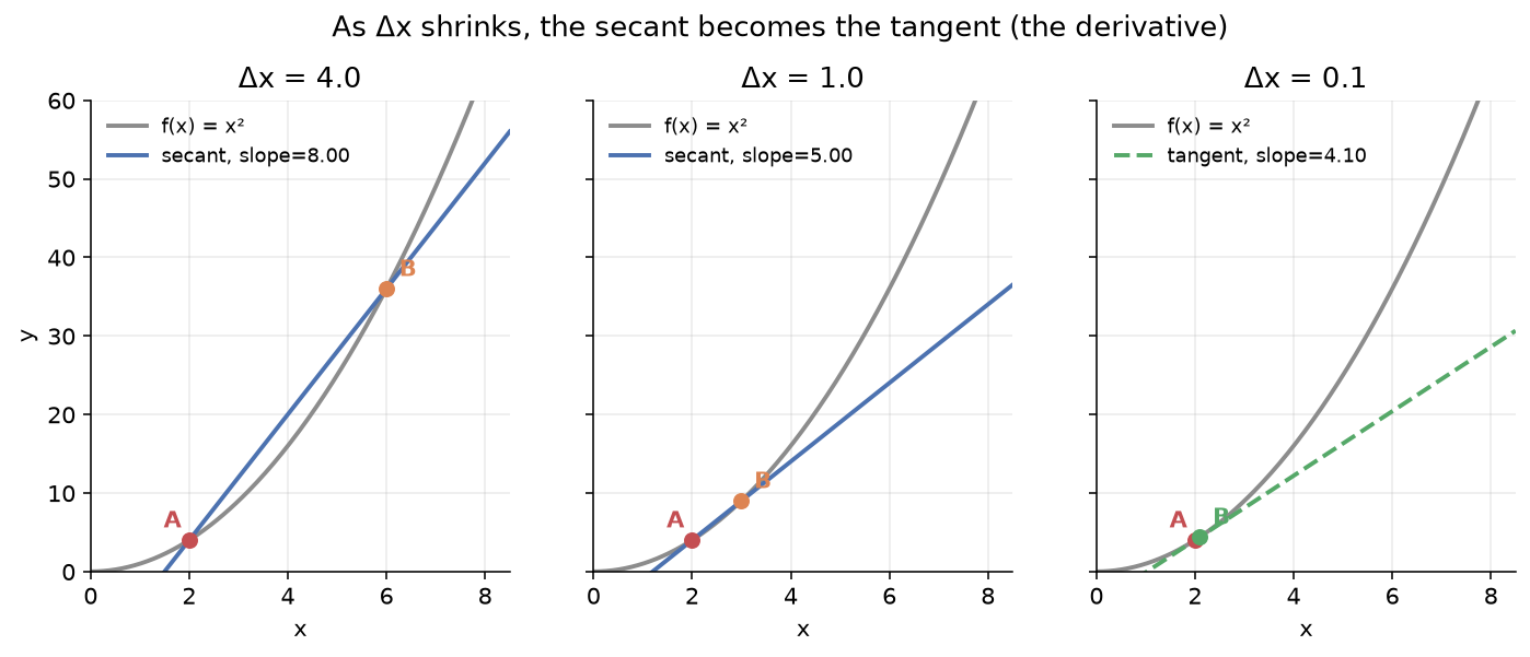
For $f(x) = x^2$ the derivative is $f'(x) = 2x$, so at $x = 2$ the slope is exactly $4$. Watch the slopes in the three panels head toward that value: $8.00, 5.00, 4.10$. The secant’s slope converges to the tangent’s slope. That is all a derivative is — the regression slope, taken to the limit.

Open the interactive demo — Section 2

Partial differentiation

Real outcomes depend on more than one variable. A toy house-price model might read

$$\text{price} = 150 \cdot \text{size} - 2000 \cdot \text{age} + 50000,$$

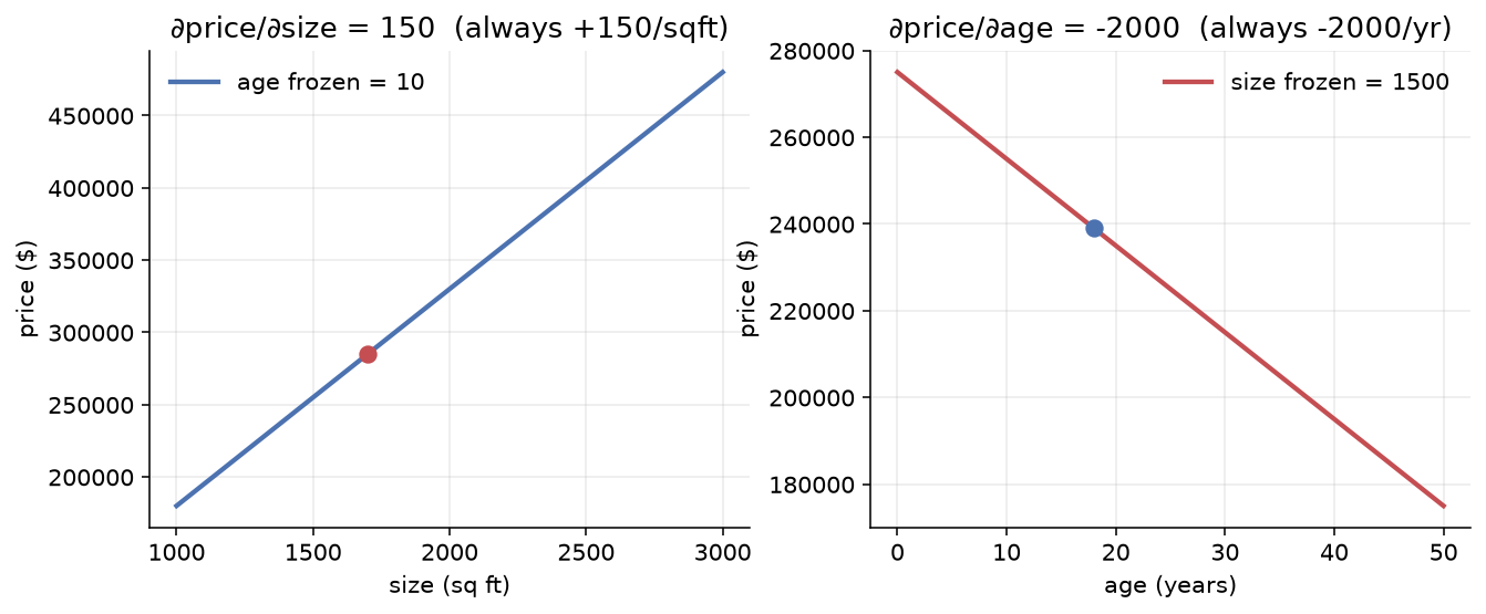
with size in square feet and age in years. Now there are two slopes to keep track of, and the question is: how does price change if I move one variable while holding the other frozen? That frozen-one-variable slope is a partial derivative, written $\partial$.

The two panels below freeze one variable each. On the left, age is held at 10 years and size varies: every extra square foot adds exactly $\$150$, so the line rises with a constant slope of $150$. On the right, size is held at 1500 sq ft and age varies: every extra year knocks off exactly $\$2000$, so the line falls. Those two numbers are the partial derivatives:

$$\partial \text{price} /\partial \text{size} = 150\$$$

and

$$\partial\text{price} / \partial \text{age} =-2000$$

They are the coefficients of the regression, spelled out.

Stack both variables on the same picture and the model is a plane in 3D — tilt it one way and price rises with size; tilt it the other and price falls with age. The current house is a single point on that plane, and the two partial derivatives are the slopes of the plane along each axis.

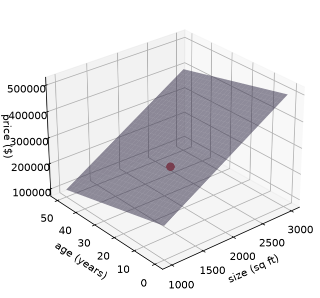
This is the leap that makes machine learning possible. With one variable we had a slope; with many variables we have a gradient — the vector of all the partial derivatives, one per parameter. The gradient points in the direction the error increases fastest, which means $-\nabla J$ points the way the error decreases fastest. That is the compass gradient descent follows.

Open the interactive demo — Section 3

Gradient descent

Now put the pieces together. We want to find the parameter value that makes the error as small as possible. The error itself is a curve — for our running example, $f(x) = x^2$ — and we are standing somewhere on it, say at $x = 8$, where the error is $64$. We cannot see the whole curve; we can only feel the slope under our feet.

The rule is the one from the opening equation: measure the slope, take a small step in the opposite direction, repeat. At $x = 8$ the slope is $2 \times 8 = 16$ — steeply uphill to the right — so we step left. With a learning rate of $\eta = 0.15$, the next position is $8 - 0.15 \times 16 = 5.6$. Slope there is $11.2$, still positive, step left again. Each step is smaller than the last, because the slope flattens as we approach the bottom. After a handful of steps we are sitting at the minimum, $x = 0$, where the slope is zero and there is nowhere lower to go.

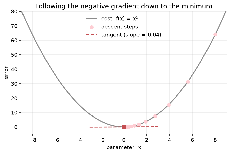
That is the entire algorithm. Every step is just subtract a scaled version of the slope. Two practical knobs matter. The learning rate $\eta$ sets the step size: too large and you overshoot the valley and bounce up the far side; too small and you crawl for ages. The convergence criterion is usually “the slope is near enough to zero” — once $|\nabla J|$ falls below a threshold, you call it done. In practice the cost curve is not a neat parabola but a high-dimensional landscape of valleys, saddles, and plateaus, which is why production training uses variants like Momentum, RMSprop, or Adam — but they are all refinements of this same rule. Step opposite to the slope. Repeat.

Open the interactive demo — Section 4

Where this goes next

The house-price model above — a weighted sum of inputs plus a bias — is, quite literally, a single artificial neuron with its activation function removed. A neuron computes the same thing:

$$z = w_1 x_1 + w_2 x_2 + \dots + w_n x_n + b$$

Strip the activation away and what is left is plain linear regression. The one “predicted price” neuron in Section 3 is the atom every neural network is built from. This is not an analogy; it is an identity. Without a non-linear activation function, even a deep stack of such layers collapses back into a single linear map, which is why activations are the thing that separates a neural network from a regression.

An activation function is a small filter applied to that weighted sum, deciding whether the neuron switches on or off, and by how much. It is a simple, bounded, non-linear function: ReLU passes positive values through and zeroes out negative ones; sigmoid squashes everything into $(0, 1)$. That single non-linearity is what gives a stack of neurons its expressive power. Stack layers of these filtered neurons together and you have the architecture behind deep learning.

Training such a network means answering, for every weight, the question: if I nudge this weight, how much does the final error change? Answering that through many stacked layers is what backpropagation does — and it is nothing more than the chain rule of calculus, applied from the output back to the input. It is the same derivative idea from Section 2, just chained through each layer so every weight learns its share of the blame for the error. The chain rule is not new mathematics; it is a 200-year-old theorem that, run in reverse on a graph of neurons, powers essentially every modern AI system.

So the chain of ideas is short, and every link is something we have already met. Regression gives the slope. Differentiation makes it instantaneous. Partial derivatives extend it to many variables at once — that vector of slopes is the gradient. Gradient descent follows the negative gradient to minimise error. Add a non-linear activation and you have a neuron; stack neurons and chain-rule their gradients and you have a neural network. Everything after this point in machine learning is a variation on that theme.

References

• Goodfellow, I., Bengio, Y., & Courville, A. Deep Learning, Chapter 4 — Numerical Computation (gradient-based optimisation) and Chapter 6 — Deep Feedforward Networks (backpropagation as the chain rule). MIT Press, 2016. https://www.deeplearningbook.org/
• Ruder, S. An overview of gradient descent optimisation algorithms. 2016. https://www.ruder.io/optimizing-gradient-descent/
• Karpathy, A. Micrograd. A tiny autograd engine that makes backpropagation (= the chain rule) readable in ~100 lines of Python. https://github.com/karpathy/micrograd
• Stanford CS231n. Optimization: Stochastic Gradient Descent and Backpropagation. https://cs231n.github.io/
• Wikipedia. Gradient descent and Backpropagation. https://en.wikipedia.org/wiki/Gradient_descent https://en.wikipedia.org/wiki/Backpropagation