Active Perception II: Adding a Visited Map to a GRU DRQN
Assets & Materials
| Active Perception — Interactive simulation. Now with two trained models selectable in the sidebar: the baseline GRU and the GRU+visited-map variant. | https://blog.vski.ai/active-perception/?model=mem |
| Active Perception I — why recurrence is the right tool when the value of the next action depends on what was just done. (Related) | https://blog.vski.ai/posts/active-perception |
| Source code and training setup for the Active Perception demo. | https://vski.sh/x/ap-demo/ |
The baseline model is a GRU Deep Recurrent Q-Network on a noisy-sensor POMDP. GRU was the starting choice for a reason: it is the cheapest recurrent cell to train, the simplest to implement, and the smallest in parameter count among the standard options. It established a working baseline at random — the model to beat while evolving the architecture.
That baseline made one load-bearing assumption that turned out to be exploitable.
The assumption was that the recurrence could carry everything sequential. Where the agent has been, what it has already swept, which direction it was facing for the last three readings — all of that was supposed to live in a 48-unit hidden state, threaded across ticks, learned end-to-end from the TD signal. This is the standard DRQN bet, and on most POMDPs it is the right bet.
On this one it leaks. The belief map zeroes its bGold and bStone
posteriors for every cell the agent has occupied (a visited cell is
certain-empty by definition), so a swept-clean cell looks to the network
identical to a never-sensed cell with a low prior. The agent can be pulled
back into already-explored territory because the input encoding cannot
distinguish “visited and empty” from “never queried.” The recurrence was
supposed to disambiguate those, and 48 hidden units on a 400-cell grid
cannot, in 3400 episodes, learn to.
The fix is one extra input tensor: a 400-bit visited bitmap, sourced from
the same shadow.confident array the renderer tints cyan. One new
projection, one new bias, no other change. It lifts the matched-pair
ratio over the baseline by and the absolute ratio vs random
from to — and the richer variant that adds the
belief channels alongside the visited bitmap loses the gain back.
That last result is the load-bearing finding here, and the reason it is worth writing up a one-tensor change.
The assumption
The Bayesian belief map is the agent’s statistical summary of the world
it has seen. Per cell, two posteriors — bGold and bStone — updated
bilaterally from each noisy reading, decaying with recency. When the
agent occupies a cell, that cell is certain-empty by construction: gold
would have been collected, stone would have blocked the move. So
ShadowBelief.markVisited sets bGold[i] = bStone[i] = 0 and flags the
cell as confident.
To the trained Q-function, the resulting (0, 0) pair is ambiguous. It
matches a never-sensed cell with a low prior exactly. The 8×4
candidate-action feature block in the observation sends the destination
cell’s (bGold, bStone, can_move, const) for each of the eight moves,
and a visited destination sends (0, 0, 1, 1) — the same vector as a
distant never-queried cell with a neutral prior.
The recurrence was supposed to fix this. The hidden state threads across ticks; in principle, the GRU cell could learn to mark “I’ve been here” into some subspace of and use it downstream. In practice, on a grid, that requires the GRU to maintain a faithful summary of a 400-bit occupancy pattern in 48 floats, learned from TD targets, in a few thousand episodes of BPTT-truncated training. It cannot. The TD signal is too sparse, the truncation window too short, the hidden state too small, the optimisation landscape too mean.
The failure mode this produces is visible in the demo. After enough ticks the agent drifts back into an already-swept region, picks up no gold there, and either escapes via the closed-form LoopGate or wastes twenty ticks re-confirming that yes, the cluster to the west really is empty. Telemetry on thirty baseline episodes shows about 30% of ticks land on a previously-visited cell. Some revisiting is unavoidable on a POMDP — the agent has to cross its own path to reach unexplored territory — but the rate is high enough to motivate giving the network the visited information directly.
The honest framing is: the recurrence is doing two jobs at once. It is learning what the recent trajectory means (good — that is what recurrence is for) and where the agent has been (bad — that is a memorisation task the cell is too small for). The fix is to offload the second job to an explicit input.
The change
The new variant adds one input tensor and one projection. Everything else — the GRU cell, the Q-head, the training loop, the Double-DQN target, the BPTT truncation, the episode replay, the potential-based shaping, the can_move mask, the LoopGate — is byte-for-byte identical to the baseline.
The third input is the visited bitmap, flattened to a 400-dim vector:
It is read off env.shadow.confident — the same Uint8Array the
renderer tints cyan and the shaping bonus integrates. No new env state.
The new projection is added inside the candidate’s pre-activation, not concatenated to the input and not appended to the Q-head:
Three design choices, each load-bearing.
Why a separate input tensor, not concatenation into . The existing input is 41-d (8-d previous-action one-hot + 33-d candidate-action features). Adding 400 more features into the same vector would inflate from to — twenty-three thousand extra parameters in three places, all of them entangled with the existing input projections, none of them with the spatial structure the map actually has. A separate projection keeps the existing weights at their validated shapes and isolates the new learning into only.
Why inside the candidate, not the Q-head. The candidate’s tanh is where the recurrence integrates “what I had” with “what I just saw.” Putting the map projection there means can incorporate “where I’ve been” into the same integration step, and the Q-head reads the result. Injecting at the Q-head instead would mean the map bypasses the recurrence entirely — a feed-forward side path that the GRU cell cannot condition on. The whole point of giving the recurrence the map is to let the recurrence use it.
Why additive, not gated. A gate would be with a learned scalar per hidden unit. It is more expressive, and it is the wrong choice here. Additive injection initialised at makes the new model’s forward pass start life numerically identical to the baseline’s — the gradient signal at step zero is “you have a new tool, here is the TD error, learn to use it.” A gate initialised at behaves the same way but adds 48 more parameters whose gradient is correlated with the recurrent tensors’, which makes the deadly triad bite harder. Additive is the smaller change that does the job.
Gradient check. The new path has its own BPTT derivative — a one-line extension of the GRU’s existing candidate gradient — and a centered finite-difference check on a tiny model passes at max relative error (float64 noise floor). The new algebra is correct.
Three variants, one decision
The natural question once “add a map” is on the table: which map? Three variants answer it.
Baseline. The shipped gru.tflite. No map input. The 41-d input
contract laid out above. Two inputs (x, h_in), two outputs
(q, h_out).
Visited-only. The variant above. One channel — the 400-bit visited
bitmap. Three inputs (x, h_in, m_in), two outputs.
parameters in over the baseline’s .
Rich. Same injection site, three channels — , flattened to 1200 dims. The hypothesis was: the recurrence also struggles to maintain a global belief summary, so giving it the full Bayesian belief alongside the visited bitmap should help at least as much as the visited bitmap alone.
The 3-arm matched-pair A/B at , 2800 episodes, three seeds shows the visited-only variant winning on every seed and the rich variant losing most of that gain back.
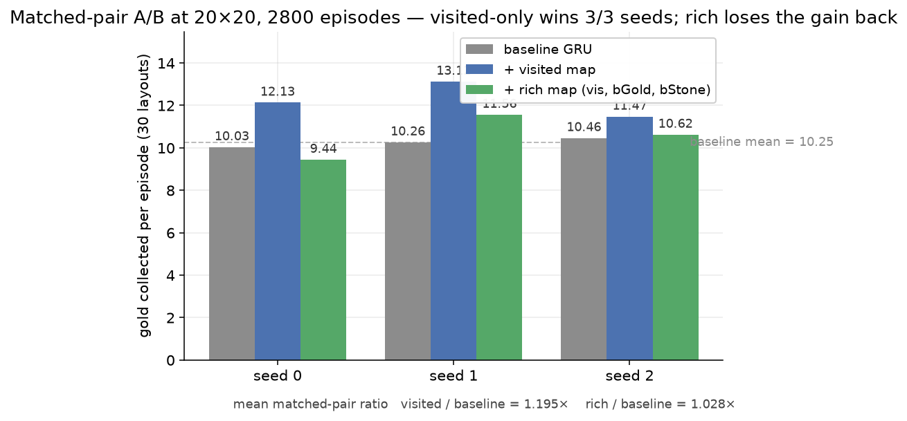
The table form, with the matched-pair ratios that matter:
| seed | baseline | visited | rich | visited / base | rich / base | rich / visited |
|---|---|---|---|---|---|---|
| 0 | 10.03 | 12.13 | 9.44 | 1.209× | 0.941× | 0.778× |
| 1 | 10.26 | 13.12 | 11.56 | 1.278× | 1.127× | 0.882× |
| 2 | 10.46 | 11.47 | 10.62 | 1.096× | 1.015× | 0.926× |
| mean | 1.194× | 1.028× | 0.862× |
The verdict is unambiguous: visited-only wins; rich does not. On seed 0 the rich variant actually loses to the baseline — adding two belief channels to the map made the agent worse than no map at all. Across the three seeds the rich variant averages the visited-only gain. The decision is visited-only.
Cross-validation
Three more checks lock the result down.
Budget sweep. The 3-arm table above is at 2800 episodes. The visited-only variant at 1400 episodes was already passing the pre-registered bar (mean matched-pair , wins on seeds), but only barely:
| budget | mean matched-pair ratio (visited / base) | seeds won |
|---|---|---|
| 1400 eps | 1.061× | 2 of 3 |
| 2800 eps | 1.194× | 3 of 3 |
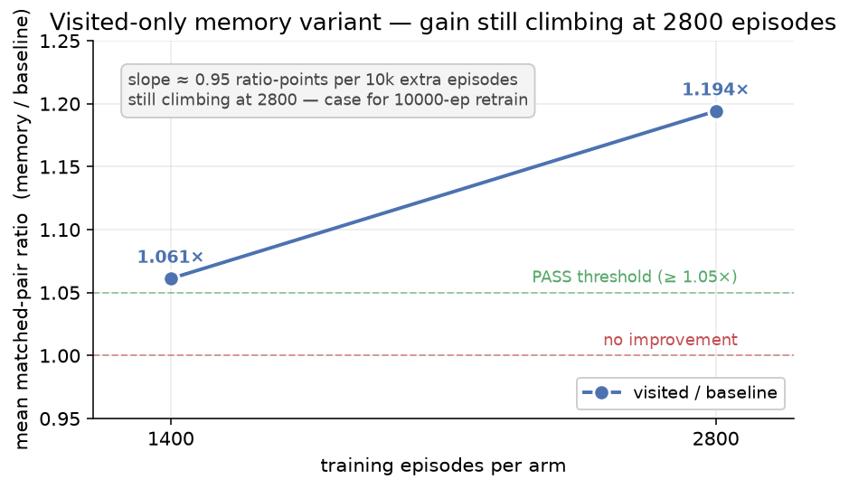
Doubling the budget tripled the gain. The curve is still climbing at 2800 — that is why the shipped artifact trains for 10000 episodes now. The honest read: at 1400 episodes the variant was under-trained, and a PASS bar of at 1400 is necessary but not sufficient to justify formalisation. Doubling the budget and seeing the gain triple is sufficient.
Behavioural read. The original hypothesis predicted the visited bitmap would reduce the revisit rate — fewer ticks landing on already-occupied cells. The metric, instrumented across thirty eval layouts:
| metric | baseline | visited | delta |
|---|---|---|---|
| collected per episode | 9.99 | 10.29 | |
| revisit rate | 30.1% | 31.5% | pp |
| unique cells visited | 112.8 | 110.2 |
What the map buys is not “stop going back” — it is better global navigation: the Q-function can now tell which regions of the grid still have unexplored clusters without trying to reconstruct that information from a 48-float hidden state. The agent spends its steps more productively, not fewer of them on revisits. That distinction matters because it tells us what to try next.
Why the richer map lost
The 3-arm A/B killed the three-channel variant by . The result is more useful than the visited-only win because it tells us what the recurrence is already doing well.
Look at what the input already gives the GRU every tick. The
candidate-action feature block sends, for each of the eight
destination cells, the destination’s (bGold, bStone, can_move, const).
That is eight local samples of the Bayesian belief map. Over a hundred
ticks the recurrence has seen the belief at every cell the agent came
close to, integrated bilaterally into the same hidden state it uses
for everything else.
Feeding the global belief map a second time, through a 57,600-parameter projection, gives the network information it has already seen in a more local form. It does not give it new information. What it does give it is a larger optimisation surface — and in 2800 episodes that surface under-fits. The visited channel is informative because the recurrence cannot reconstruct it from local samples (it would need to remember every cell it has occupied, which is the original problem). The belief channels are redundant because the recurrence already has them, locally, in the same form.
This is a textbook “more capacity, less signal” failure. The lesson generalises: before adding an input modality to a recurrent value function, ask whether the recurrence is already implicitly tracking that modality. If yes, the extra input is parameter inflation that hurts optimisation. If no — as with the visited bitmap — the extra input is genuinely new signal and the recurrence will use it.
Where a CNN would be the right next step
The visited bitmap is a flat 400-dim vector through a dense projection. That projection treats every cell as independent of every other cell — the parameter does not know or care that cell and cell are spatially adjacent. For “is this cell visited” that is fine; a per-cell binary feature has no spatial structure worth exploiting.
But the moment the map carries information whose spatial layout matters, a dense projection is the wrong tool. Three concrete situations where the next architectural step is a small convolutional encoder on the map input, not another dense projection:
When the agent should reason about region shape, not per-cell state. “Is there a contiguous unexplored corridor to the east” is a spatial question — the answer depends on a run of unvisited cells in the same direction, not on any individual cell. A two- or three-layer convolutional encoder with kernels learns exactly these local-spatial motifs; a dense projection cannot, without vastly more parameters and a much longer training schedule. The visited bitmap in this demo is on the edge of benefiting from this — there is mild spatial structure in “runs of unvisited cells” — which is why the dense projection works but is not obviously optimal.
When the map carries graded spatial signals. The Bayesian
posteriors bGold and bStone are graded — a cell can be “probably
gold”, “maybe gold”, “unknown”, “probably empty” — and the spatial
pattern of those grades is informative. A cluster of high-bGold
cells surrounded by unknown ones is a different signal from a single
high-bGold cell surrounded by certain-empties. Convolutions extract
exactly this kind of neighbourhood statistic. The rich variant in
the 3-arm A/B tried to give the network those graded signals through
a dense projection and lost; the right retry is a small conv encoder
on the (visited, bGold, bStone) stack. The failure of the dense
rich variant is not evidence that the information is useless — it is
evidence that the dense encoder is the wrong reader for it.
When the agent has to act at a different scale than it senses. If the grid were instead of , a dense projection would be parameters just for the map input — most of the model. A convolutional encoder with shared weights scales with map area in compute, not in parameters. This is the standard argument for convolutions anywhere the input has a regular grid topology, and it applies here as soon as the grid scales.
What a CNN does not fix is the recurrence’s job. The recurrent cell still has to integrate the CNN’s map summary with the per-tick trajectory features and decide what to do next. A CNN encoder feeding a GRU value head is a different architecture — closer to a visual-DQN hybrid than a pure DRQN — and it brings its own stabilisation headaches (the deadly triad bites harder as the value function gets more expressive). The right experiment is a and conv stack on the map input, the visited-only variant as the A/B baseline, and a matched-pair test on at least 5000 episodes per arm. If the conv variant wins by on seeds, formalise. If it does not, the dense visited projection is the right tool and the spatial structure of this particular map is not load-bearing.
Conclusion
A GRU DRQN whose recurrence cannot carry one specific piece of sequential state benefits from having that state fed in explicitly, even if the explicit input is just a binary bitmap. The bitmap is one extra tensor, one extra projection, one extra line in the candidate’s pre-activation. The matched-pair gain is at three seeds and three-thousand episodes per arm; the production retrain lifts the absolute ratio from random to .
When the map input graduates from “binary occupancy” to “graded spatial fields” — belief posteriors, reward gradients, sensor confidence — the dense projection is the wrong reader. A small convolutional encoder respects the spatial structure the dense projection flattens away, and scales with grid area in compute rather than parameters. The right next experiment is a convolutional map encoder against the visited-only baseline, same matched-pair protocol, same PASS bar.
The architecture that follows is one line different from the baseline: the GRU cell gets a third input tensor and the candidate’s pre-activation picks up a tanh-projected map summary. Everything else — the training pipeline, the LoopGate, the deployment recipe — is unchanged. The discipline that got us here: diagnose the failure mode, fix it at the smallest layer that addresses it, validate at three seeds before formalising.
References
- Active Perception I — A GRU DRQN for Discovery Under a Noisy Sensor. The baseline model this work evolves. A GRU DRQN on the same noisy-sensor POMDP, with the regime, the architecture, and the mask-on-top-of-frozen-policy deployment recipe that the visited-map variant inherits unchanged.
- Hausknecht, M. & Stone, P. Deep Recurrent Q-Learning for Partially Observable MDPs. (arXiv.06527, 2015) — the DRQN recipe (truncated BPTT, episode replay) this variant inherits. The architecture change here is one extra input tensor; the training loop is identical.
- Mnih, V. et al. Human-level control through deep reinforcement learning. (Nature 518, 2015) — the DQN stabilisers (target network, replay, function approximation under the deadly triad) that any nonlinear value-function change has to preserve.
- Cho, K. et al. Learning Phrase Representations using RNN Encoder-Decoder for Statistical Machine Translation. (EMNLP 2014) — the GRU cell equations extended here with one extra additive term in the candidate.
- LeCun, Y. et al. Gradient-Based Learning Applied to Document Recognition. (Proc. IEEE 1998) — the case for convolutional encoders on inputs with regular grid topology. The right reader for a graded spatial map, as opposed to the dense projection that works for a binary occupancy bitmap.
- Executable companion.
Active Perception demo —
the baseline GRU and the GRU+visited-map variant side by side,
selectable in the sidebar. Both ship as frozen
.tflites; both compose with the same LoopGate.